1. Background

Ambient noise tomography has been a very popular imaging strategy of investigating the earth’s interior in past over two decades. The basic principle of this method is that stacked cross-correlations from noise recordings made by two receivers can be approximately the Green’s function from one receiver to another. We have the need of synthesizing ambient noise for validating this important idea, or exploring characteristics of ambient noise. Here we introduce a simple way of computing synthetic ambient noise.

2. Steps to doing synthetics

2.1 Configuring the receiver and source positions

Firstly we randomly generate source and receiver positions with given coordinate ranges using the following python codes:

 1
 2
 3
 4
 5
 6
 7
 8
 9
10
11
12
13
14
15
import numpy as np
import matplotlib.pyplot as plt
nr = 60
r = 250
th = np.linspace(0, 2*np.pi, nr)
ra = np.linspace(0, r, nr)
xy = np.zeros((nr, 2))
xy[:, 0] = ra * np.cos(th)
xy[:, 1] = ra * np.sin(th)
xy[:, 0] += (np.random.randn(nr) * 100)
xy[:, 1] += (np.random.randn(nr) * 100)
plt.figure(figsize=(6, 6))
plt.plot(xy[:, 0], xy[:, 1], 'bv', alpha=0.5)
plt.show()
np.savetxt('rec.txt', xy)

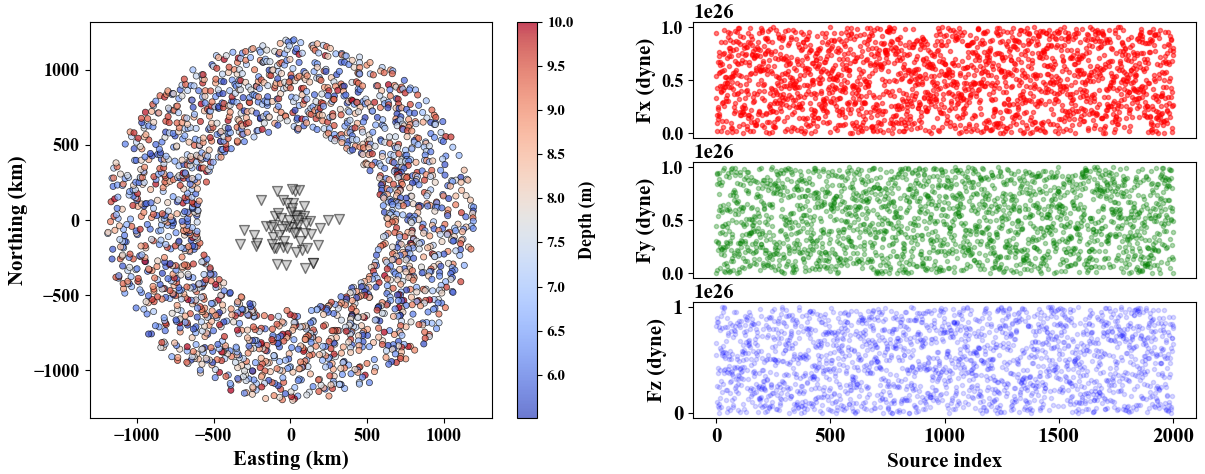
We generated 60 receivers within the circle with radius of ~250 km, and coordinates are saved in rec.txt. Now we generate 2001 sources within a ring belt with radius limitations of 600 km and 1200km, and three-component forces. Note that source positions are stored in file src.txt, and force components are saved in file force.txt.

 1
 2
 3
 4
 5
 6
 7
 8
 9
10
11
12
13
14
15
16
17
18
import numpy as np
import matplotlib.pyplot as plt

rxy = np.loadtxt('rec.txt')
r1 = 600; r2 = 1200
d1 = 1e-3; d2 = 1e-2
ns = 2001
th = np.linspace(0, 2*np.pi, ns)
r = np.random.random(ns)
dep = np.random.random(ns)
r /= np.abs(r).max()
r = r1 + r*(r2-r1)
dep = dep / np.abs(dep).max()
dep += 1
dep /= np.abs(dep).max()
dep = d1 + dep*(d2-d1)
force = np.random.random((ns, 3)) * 1.0e26
np.savetxt('force.txt', force)

The receiver and source configuration is shown by the following figure.

 1
 2
 3
 4
 5
 6
 7
 8
 9
10
11
12
13
14
15
16
17
18
19
20
21
22
23
24
25
26
27
28
29
30
31
32
33
34
import numpy as np
import matplotlib.pyplot as plt
from obspy import read

xy = np.loadtxt('rec.txt')
sr = np.loadtxt('src.txt')
f = np.loadtxt('force.txt')
plt.figure(figsize=(14, 5.5))
ax1 = plt.subplot(121)
ax1.scatter(xy[:, 0], xy[:, 1], s=50, marker='v',
            facecolor='#AAAAAA', edgecolor='k', lw=1, alpha=0.5)
plt.scatter(sr[:, 0], sr[:, 1], s=20, c=sr[:, 2]*1e3, marker='o', cmap='coolwarm',
            facecolor='#AAAAAA', edgecolor='k', lw=0.5, alpha=0.75)
cbar = plt.colorbar()
cbar.ax.tick_params(labelsize=11)
cbar.set_label('Depth (m)', fontsize=13)
ax1.tick_params(labelsize=13)
ax1.set_xlabel('Easting (km)', fontsize=15)
ax1.set_ylabel('Northing (km)', fontsize=15)
ax2 = plt.subplot(3, 2, 2)
ax2.plot(f[:, 0], 'r.', alpha=0.50)
ax2.set_ylabel('Fx (dyne)', fontsize=15)
ax2.tick_params(labelsize=13)
ax2.set_xticks([])
ax3 = plt.subplot(3, 2, 4)
ax3.plot(f[:, 1], 'g.', alpha=0.30)
ax3.set_ylabel('Fy (dyne)', fontsize=15)
ax3.tick_params(labelsize=13)
ax3.set_xticks([])
ax4 = plt.subplot(3, 2, 6)
ax4.plot(f[:, 2], 'b.', alpha=0.15)
ax4.set_xlabel('Source index', fontsize=15)
ax4.set_ylabel('Fz (dyne)', fontsize=15)
plt.show()

REC-SRC

2.2 Synthetic ambient noise

The ambient noise recordings can be considered as the wavefield excited by many events, like the primary and secondary microseisms from interactions between ocean waves and our solid earth, and maybe some weak seismic signals generated by small earthquakes. These events randomly occur in time and space. Therefore, we compute seismic waveforms triggered by many earthquakes, and randomly stack these earthquake-generated waveforms according to event occuring time and their positions. Finally we synthesize ambient seismic noise. The python codes of computing waveforms excited by earthquakes:

 1
 2
 3
 4
 5
 6
 7
 8
 9
10
11
12
13
14
15
16
17
18
19
20
21
22
23
24
25
26
27
28
29
30
31
32
33
34
35
36
37
38
39
40
41
42
import numpy as np
import os

# read in source and receiver position information.
src = np.loadtxt('src.txt')
rec = np.loadtxt('rec.txt')
nr = rec.shape[0]
evt_dir = 'event/'
if not os.path.exists(evt_dir):
    os.mkdir(evt_dir)
for i in range(nr):
    sta = evt_dir + 'station_%02d'%(i+1)
    if not os.path.exists(sta):
        os.mkdir(sta)
nmode = 3
ns = src.shape[0]
# read in three-component forces.
force = np.loadtxt('force.txt')
fx = force[:, 0]
fy = force[:, 1]
fz = force[:, 2]
# compute synthetic waveforms
for i in range(ns):
    sx, sy, dep = src[i]
    tag_s = i + sn1 + 1
    for j in range(nr):
        dx = sx - rec[j, 0]; dy = sy - rec[j, 1]
        dist = ( dx**2 + dy**2 ) ** 0.5
        az = np.pi/2 - np.arctan2(dy, dx)
        az = az * 180 / np.pi
        dfile = '%g 0.25 2048 0 0'%dist
        with open('dfile', 'w') as fout:
            fout.write(dfile)
        os.system('sprep96 -M model.md -NMOD %d -HS %g -HR 0 -d dfile -R'%(nmode, dep))
        os.system('sdisp96')
        os.system('sregn96')
        os.system('spulse96 -d dfile -D -i -ALL -2 > file96')
        os.system('fmech96 -A %g -fx %f -fy %f -fz %f -ROT < file96 > tosac.file'%(az, fx[i], fy[i], fz[i]))
        os.system('f96tosac -B tosac.file')
        os.system('mv B00101Z00.sac %s/station_%02d/%04d.Z.%02d.SAC'%(evt_dir, j+1, tag_s, j+1))
os.system('rm *R00.sac')
os.system('rm file96 sdisp96.dat sregn96.egn tosac.file sdisp96.ray')

Now we synthesize ambient noise with the following codes:

 1
 2
 3
 4
 5
 6
 7
 8
 9
10
11
12
13
14
15
16
17
18
19
20
21
22
23
24
25
26
27
28
29
30
31
32
33
34
35
36
37
38
39
40
41
42
43
44
45
46
47
48
49
import numpy as np
from obspy import read
from obspy.core import Trace, AttribDict
from glob import glob
import os

evt_dir = 'event/'
noise_dir = 'noise/'
if not os.path.exists(noise_dir):
    os.mkdir(noise_dir)

print('Read in event data ...')
st = []
nr = 60
ns = 2001
for i in range(1, nr+1):
    st.append(read('%sstation_%02d/*.Z.*.SAC'%(evt_dir, i)))
print(len(st), len(st[0]))


print('Synthesize noise data ...')
dt = st[0][0].stats.delta
ns = len(st[0])
nd = len(st[0][0].data)
n = nd * 500
data = np.zeros((nr, n))
index = np.random.random(ns*50)
index /= index.max()
for i in range(len(index)):
    si = int(index[i]*ns)
    if si >= ns:
        si = ns - 1
    ti = int(np.random.random()*n)
    if ti > n - 1 - nd:
        ti = n - 1 - nd
    for j in range(nr):
        data[j, ti: ti+nd] += st[j][si].data

for i in range(nr):
    data[i] /= np.abs(data[i]).max()
print('Write out noise data ...')
t = np.arange(n) * dt
sac = Trace(t)
sac.stats.sac = AttribDict({})
sac.stats.delta = dt
sac.stats.sac.b = 0
for i in range(nr):
    sac.data = data[i]
    sac.write('%snoise.Z.%02d.SAC'%(noise_dir, i+1), format='SAC')

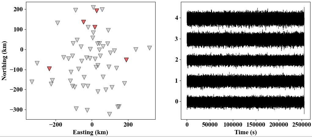
We randomly choose synthetic ambient noise waveforms from 5 receivers to visualize:

 1
 2
 3
 4
 5
 6
 7
 8
 9
10
11
12
13
14
15
16
17
18
19
20
21
22
23
24
25
26
27
28
29
30
31
import numpy as np
import matplotlib.pyplot as plt
from obspy import read
nr = 60
n = 5
index = []
for i in range(200):
    if len(index) >= n:
        break
    ri = int(np.random.random() * nr)
    if ri not in index:
        index.append(ri)
xy = np.loadtxt('rec.txt')

plt.figure(figsize=(12, 5))
plt.subplot(121)
plt.scatter(xy[:, 0], xy[:, 1], s=100, marker='v',
            facecolor='#AAAAAA', edgecolor='k', lw=1, alpha=0.5)
plt.scatter(xy[index, 0], xy[index, 1], s=100, marker='v',
            facecolor='r', edgecolor='k', lw=1, alpha=0.5)
plt.xlabel('Easting (km)')
plt.ylabel('Northing (km)')
plt.subplot(122)
for i in range(n):
    tr = read('noise/noise.Z.%02d.SAC'%(index[i]+1))[0]
    dt = tr.stats.delta
    data = tr.data
    t = np.arange(len(data)) * dt
    plt.plot(t, data*0.6+i, lw=0.5, color='k')
plt.xlabel('Time (s)')
plt.show()

SYN-NOISE

3. Checking the relation between receiver-pair cross-correlation and the green’s function

Ideal source distribution (energy equipartion in all directions) can lead to the phase smilarity between stacked cross-correlations and the Green’s functions. For detail, the relation is given by $$ G_{AB}(t) = -\frac{dC_{AB}(t)}{dt}=\frac{dC_{AB}(-t)}{dt}, \tag{1} $$ where, $G_{AB}(t)$ and $C_{AB}(t)$ are separately the Green’s function and stacked cross-correlation between receiver A and B. Now we compute the temporally average cross-correlation function between receivers.

 1
 2
 3
 4
 5
 6
 7
 8
 9
10
11
12
13
14
15
16
17
18
19
20
21
22
23
24
25
26
27
28
29
30
31
32
33
34
35
36
37
38
39
40
41
42
43
44
45
46
47
48
49
50
51
52
53
54
55
56
57
58
import numpy as np
from obspy import read
from obspy.core import Trace, AttribDict
import os

rxy = np.loadtxt('rec.txt')
st = read('noise/noise*.SAC')
nr = len(st)

dt = st[0].stats.delta
# ccf time window length and movement window length
segt = 2000; pt = 1000
segn = int(segt/dt)
pn = int(pt/dt)
data = np.zeros((nr, st[0].stats.npts))
print(st[0].stats.npts, data.shape)
for i in range(nr):
    data[i] = st[i].data

ccf_dir = 'ncf_%s/'%(noise.split('_')[-1][:-1])
if not os.path.exists(ccf_dir):
    os.mkdir(ccf_dir)

nfft = 2 * segn - 1
operator = np.ones(5) / 5
cfd = np.zeros(nfft, dtype=complex)
ct = np.arange(nfft) * dt - nfft//2 * dt

cor = Trace(ct)
cor.stats.delta = dt
cor.stats.sac = AttribDict({})
cor.stats.sac.b = ct[0]
cor.stats.sac.lcalda = True
# frequency band of ccf
f1 = 0.01; f2 = 0.6
for i in range(nr-1):
    for j in range(i+1, nr):
        ccf = ccf_dir + 'ccf_%02d_%02d.SAC'%(i+1, j+1)
        print(ccf)
        dist = ( (rxy[i][0]-rxy[j][0])**2 + (rxy[i][1]-rxy[j][1])**2 ) ** 0.5
        cor.stats.sac.dist = dist
        cfd = np.zeros(nfft, dtype=complex)
        nn = 0
        while nn < st[0].stats.npts - segn:
            dd1 = data[i, nn: nn+segn].copy()
            dd2 = data[j, nn: nn+segn].copy()
            dd1 -= dd1.mean(); dd2 -= dd2.mean()
            fd1 = np.fft.fft(dd1, nfft)
            fd2 = np.fft.fft(dd2, nfft)
            fd1 /= np.convolve(np.abs(fd1), operator, 'same')
            fd2 /= np.convolve(np.abs(fd2), operator, 'same')
            fd1[np.isnan(np.abs(fd1))] = 0.
            fd2[np.isnan(np.abs(fd2))] = 0.
            cfd += (fd1 * np.conjugate(fd2))
            nn += pn
        cor.data = np.fft.ifftshift(np.fft.ifft(cfd)).real
        cor.filter('bandpass', freqmin=f1, freqmax=f2, corners=4, zerophase=True)
        cor.write(ccf, format='SAC')

Here we compare the empirical green’s function from cross-corrlation and corresponding Green’s function with distance of ~ 500 km on different frequency bands.

 1
 2
 3
 4
 5
 6
 7
 8
 9
10
11
12
13
14
15
16
17
18
19
20
21
22
23
24
25
26
27
28
29
30
31
32
33
34
import numpy as np
import matplotlib.pyplot as plt
from obspy import read
tr1 = read('ncf_01/ccf_14_41.SAC')[0]
tr1.differentiate()
tr1.data *= (-1)
tr2 = read('B00102R00.sac')[0]
T = [[2, 5], [5, 10], [10, 20], [15, 50], [20, 100]]
plt.figure(figsize=(10, 8))
for i in range(len(T)):
    T1 = T[i][0]; T2 = T[i][1]
    f1 = 1 / T2; f2 = 1 / T1
    trc1 = tr1.copy()
    trc1.filter('bandpass', freqmin=f1, freqmax=f2, corners=4, zerophase=True)
    trc2 = tr2.copy()
    trc2.filter('bandpass', freqmin=f1, freqmax=f2, corners=4, zerophase=True)
    d1 = trc1.data; d1 /= np.abs(d1).max()
    d2 = trc2.data; d2 /= np.abs(d2).max()
    tt1 = np.arange(len(d1)) * tr1.stats.delta + tr1.stats.sac.b
    tt2 = np.arange(len(d2)) * tr2.stats.delta + tr2.stats.sac.b
    plt.subplot(len(T), 1, i+1)
    plt.plot(tt1, d1, 'r', lw=2, alpha=0.5, label='EGF')
    plt.plot(tt2, d2, 'b', lw=2, alpha=0.35, label='GF')
    plt.xlim(0, 300)
    if i < 4:
        plt.xticks([])
    if i < 1:
        plt.title('Dist.: %.3f km  Period: %d-%d s'%(tr1.stats.sac.dist, T1, T2), fontsize=13)
        plt.legend(fontsize=12, loc='upper right')
    else:
        plt.title('Period: %d-%d s'%(T1, T2), fontsize=13)
    plt.gca().tick_params(labelsize=12)
plt.xlabel('Time (s)', fontsize=15)
plt.show()

CCF-GF 
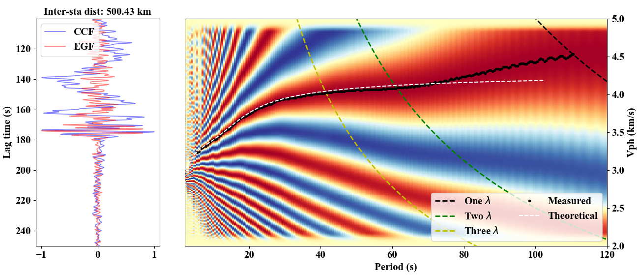
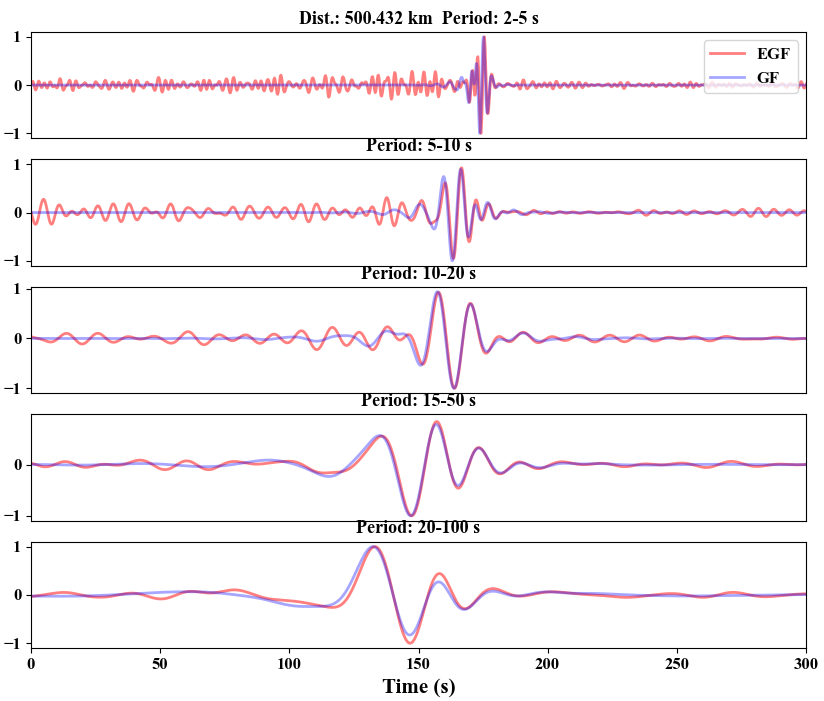
The cross-correlation and Green’s function waveforms are very similar on different period ranges. Furthermore, we use the image transform technique (Yao et al., 2006) to estimate dispersion curve from the cross-correlation function, and compare it with the theoretical one.

  1
  2
  3
  4
  5
  6
  7
  8
  9
 10
 11
 12
 13
 14
 15
 16
 17
 18
 19
 20
 21
 22
 23
 24
 25
 26
 27
 28
 29
 30
 31
 32
 33
 34
 35
 36
 37
 38
 39
 40
 41
 42
 43
 44
 45
 46
 47
 48
 49
 50
 51
 52
 53
 54
 55
 56
 57
 58
 59
 60
 61
 62
 63
 64
 65
 66
 67
 68
 69
 70
 71
 72
 73
 74
 75
 76
 77
 78
 79
 80
 81
 82
 83
 84
 85
 86
 87
 88
 89
 90
 91
 92
 93
 94
 95
 96
 97
 98
 99
100
101
import numpy as np
import matplotlib.pyplot as plt
from scipy.interpolate import CubicSpline
from scipy.signal import hilbert, hann
from obspy import read

tr = read('ncf_01/ccf_14_41.SAC')[0]
d0 = tr.data.copy()
tr.differentiate()
tr.data *= (-1)
T1 = 2
T2 = 120
gv1 = 2
gv2 = 5
dt = tr.stats.delta
b = tr.stats.sac.b
gcarc = tr.stats.sac.dist
t1 = gcarc / gv2
t2 = gcarc / gv1
n1 = int((t1-b)/dt); n2 = int((t2-b)/dt)
nt = n2 - n1 + 1
tr.data[:n1] = 0
tr.data[n2:] = 0
d = tr.data[n1: n2+1]
t = np.arange(nt) * dt + t1

dT0 = 0.5
T = np.arange(T1, T2+dT0, dT0)
nT = len(T)
dT = 0.25
ng = 251
dv = 0.2
p = np.zeros((ng, nT))
vph = np.linspace(gv1, gv2, ng)
dn = int(dv/(vph[1]-vph[0]))
h = hann(2*dn)
for i in range(nT):
    dTT = dT
    f1 = 1 / (T[i]+dTT)
    f2 = 1 / (T[i]-dTT)
    trc = tr.copy()
    trc.filter('bandpass', freqmin=f1, freqmax=f2, corners=4, zerophase=True)
    d = trc.data[n1: n2+1]
    d /= abs(d).max()
    tmp = gcarc/(t-T[i]/8)
    index = np.argsort(tmp)
    natural = CubicSpline(tmp[index], d[index], bc_type='natural')
    p[:, i] = natural(vph, nu=0)
    p[:dn, i] *= h[:dn]; p[-dn:, i] *= h[dn:]
    p[:, i] /= np.abs(p[:, i]).max()
    p[:dn, i] *= h[:dn]; p[-dn:, i] *= h[dn:]
d0 /= np.abs(d0).max()
d1 = tr.data; d1 /= np.abs(d1).max()

fig = plt.figure(figsize=(15, 6))
ax1 = plt.subplot2grid((1, 4), (0, 0), rowspan=1, colspan=1)
ax1.plot(d0[n1: n2+1], t, lw=1.25, color='b', alpha=0.5, label='CCF')
ax1.plot(tr.data[n1: n2+1], t, lw=1.25, color='r', alpha=0.5, label='EGF')
ax1.legend()
ax1.set_ylabel('Lag time (s)')
ax1.set_title('Inter-sta dist: %.2f km'%gcarc)
ax1.set_ylim(t[0], t[-1])
ax1.invert_yaxis()

ax2 = plt.subplot2grid((1, 4), (0, 1), rowspan=1, colspan=3)
ax2.pcolormesh(T, vph, p, cmap='RdYlBu_r')
ax2.plot(T, gcarc/T, 'k--', lw=2, label='One $\lambda$')
ax2.plot(T, gcarc/T/2, 'g--', lw=2, label='Two $\lambda$')
ax2.plot(T, gcarc/T/3, 'y--', lw=2, label='Three $\lambda$')
ax2.set_xlabel('Period (s)')
ax2.set_ylabel('Vph (km/s)')
ax2.set_xlim(T1, T2)
ax2.set_ylim(gv1, gv2)
ax2.yaxis.set_label_position('right')
ax2.yaxis.set_ticks_position('right')

dv = 0.075; r = 1.0
tmp = [5.7, 3.253]
if len(tmp) < 1:
    plt.close()
    sys.exit(1)
    plt.close()
t0, v0 = tmp
print(t0, v0)
tn0 = int((t0-T.min())/(T[1]-T[0])+0.5)
vn0 = int((v0-vph.min())/(vph[1]-vph[0])+0.5)
vi = vn0
vm = []
for i in range(tn0, nT):
    dvn = int(dv/(vph[1]-vph[0])+0.5)
    pi = np.argmax(p[vi-dvn: vi+dvn, i])
    vi = vi - dvn + pi
    vm.append([T[i], vph[vi]])
    if gcarc/T[i]*r < vph[vi]:
        break
vm = np.array(vm)
ax2.plot(vm[:, 0], vm[:, 1], 'k.', lw=2, label='Measured')
dc = np.loadtxt('disp.txt')
ax2.plot(1/dc[:, 0], dc[:, 1], 'w--', label='Theoretical')
plt.legend(loc='lower right', fontsize=15, ncol=2)
plt.show()

CCF_DC

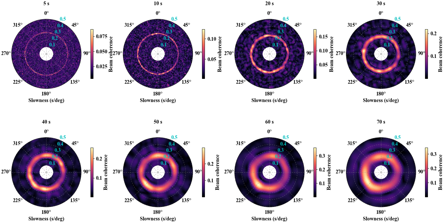
4. Noise source distribution from beamforming analysis

We utilize the beamforming array method to detect back-azimuth and slowness of noise sources to explore whether these sources come from all directions.

 1
 2
 3
 4
 5
 6
 7
 8
 9
10
11
12
13
14
15
16
17
18
19
20
21
22
23
24
25
26
27
28
29
30
31
32
33
34
35
36
37
38
39
40
41
42
43
44
45
46
47
48
49
50
51
52
53
54
55
56
57
58
59
60
61
62
63
64
65
66
import numpy as np
import matplotlib.pyplot as plt
from scipy import fft
from obspy import read
from glob import glob
import re

rxy = np.loadtxt('rec.txt') * 1e3
files = sorted(glob('ncf_01/*.SAC'))
ccf = []
pos = []
t0 = 250
t1 = -t0; t2 = t0
for sac in files:
    tmp = re.split(r'[_|.]', sac.split('/')[-1])
    ri1 = int(tmp[1]); ri2 = int(tmp[2])
    tr = read(sac)[0]
    x1, y1 = rxy[ri1-1]
    x2, y2 = rxy[ri2-1]
    b = tr.stats.sac.b; dt = tr.stats.delta
    n1 = int((t1-b)/dt); n2 = int((t2-b)/dt)
    d = tr.data[n1: n2+1]; n = len(d)
    fd = fft.fft(d)
    ccf.append(fd); pos.append([x2-x1, y2-y1])
ccf = np.array(ccf); pos = np.array(pos)

nf = ccf.shape[1]; fs = 1 / dt
fre = np.arange(nf) * fs / nf
s1 = 1e-4; s2 = 5e-4
sn = 81; bn = 181
slow = np.linspace(s1, s2, sn)
baz = np.radians(np.linspace(0, 360, bn))
bazz = baz - np.pi

T = [5, 10, 20, 30, 40, 50, 60, 70]
dT = [0.1] * 8
plt.figure(figsize=(16, 9))
for ti in range(len(T)):
    print('Period of %d s ...'%T[ti])
    f1 = 1 / (T[ti]+dT[ti]); f2 = 1 / (T[ti]-dT[ti])
    fn1 = np.argmin(np.abs(fre-f1))
    fn2 = np.argmin(np.abs(fre-f2))
    p = np.zeros((sn, bn))
    for fn in range(fn1, fn2+1):
        ff = fre[fn]
        cf = ccf[:, fn]
        cf /= np.abs(cf); cf[np.isnan(np.abs(cf))] = 0.
        tmp = -2j * np.pi * ff
        for i, ss in enumerate(slow):
            for j, bb in enumerate(bazz):
                shift = ss * (np.sin(bb)*pos[:, 0] + np.cos(bb)*pos[:, 1])
                p[i, j] += np.abs(np.dot(cf, np.exp(tmp*shift)))
    p = p / cf.shape[0] / (fn2-fn1+1)
    ax = plt.subplot(2, 4, ti+1, projection='polar')
    plt.pcolormesh(baz, slow*1e3, p, cmap='magma')
    cbar = plt.colorbar(shrink=0.5, pad=0.1)
    cbar.set_label(r'Beam coherence', fontsize=13)
    cbar.ax.tick_params(labelsize=13)
    ax.grid(color='gray', ls=(10, (6, 5)), lw=0.5)
    ax.tick_params(axis='y', colors='c', labelsize=13)
    ax.set_theta_zero_location('N')
    ax.set_theta_direction(-1)
    ax.set_xlabel('Slowness (s/deg)', fontsize=13)
    plt.xticks(fontsize=13); plt.yticks(fontsize=13)
    plt.title('%d s'%(T[ti]), fontsize=13, pad=15)
plt.show()

BEAM

References

Yao, H., R. D. van der Hilst, and M. V. de Hoop (2006), Surface-wave array tomography in SE Tibet from ambient seismic noise and two-station analysis—I. Phase velocity maps, Geophys. J. Int., 166, 732 – 744, doi:710.1111/j.1365-1246X.2006.03028.x