Background

Ambient noise tomography is widely used to image th earth’s interior in past over two decades for various scales. Stacked cross-correlations from seismic ambient noise can be approxmately the Green’s functions between receivers. Surface waves extracted from ambient noise cross-correlations are frequently utilized to estimate multi-layered shear wave velocity structure. The key to surface wave imageing is reliable dispersion curves. Two-staion techniques, like frequency-time analysis (Levshin et al., 1989), image transform (Yao et al., 206) and zero-crossing (Ekstrom et al., 2009), are popular methods of extracting dispersion curves. Here we introduce the image transform technique for estimating surface wave phase velocity dispersion curves.

Basic principles

In order to satisfy the far-field approximation, we require the epicentral distance $\Delta$ to be three times of the largest wavelength of considered harmonic signals. The phase traveltime $t$ from source A to receiver B holds $$ k_{AB} - \omega t + \frac{\pi}{4}=0, \tag{1} $$ where, $k_{AB}$ and $\omega$ are wavenumber and angular frequency of signal traveling from A to B. Using relation $\omega=2\pi/T$ and $k_{AB}=2\pi/T/c_{AB}$The average phase velocity $c_{AB}$ between A and B is given by $$ c_{AB} = \frac{\Delta}{t-T/8}, \tag{2} $$ in which, $T$ is the period.

Numerical examples

We use the CPS package (https://www.eas.slu.edu/eqc/eqc_cps/getzip.html) to compute vertical and radial component Green’s functions to check the reliability of estimating dispersion curve using the image transform technique. Suppose that the shell script file name is run_syn_sac.sh containing the following shell codes:

 1
 2
 3
 4
 5
 6
 7
 8
 9
10
11
12
HS=0.001
NMODE=1
AZ=${4}
awk 'BEGIN{for(i='''${2}''';i<='''${3}''';i++) print i*'''${1}''',"0.125 4096 0 0"}' > dfile
sprep96 -M model.md -NMOD ${NMODE} -HS ${HS} -HR 0 -d dfile -R -L
sdisp96
sregn96
slegn96
sdpegn96 -R -C -PER -TXT -XLOG -YMIN 1 -YMAX 5
spulse96 -d dfile -D -i -EX -2 > file96
fmech96 -ROT -A ${AZ} -fz -1.0e26 < file96 > tosac.file
f96tosac -B tosac.file

Note that you should prepare a model file model.md for doing synthetics:

 1
 2
 3
 4
 5
 6
 7
 8
 9
10
11
12
13
14
15
16
17
18
19
20
21
22
23
24
25
26
27
MODEL
US MODEL
ISOTROPIC
KGS
SPERICAL EARTH
1-D
CONSTANT VELOCITY
LINE08
LINE09
LINE10
LINE11
H VP VS RHO QP QS ETAP ETAS FREFP FREFS
5  5.516227 3.252661 2.585847  0 0 0 0 1. 1.
5  6.268066 3.661441 2.776762  0 0 0 0 1. 1.
5  6.463846 3.761447 2.824013  0 0 0 0 1. 1.
5  6.357846 3.707419 2.798076  0 0 0 0 1. 1.
5  6.893768 3.978853 2.937814  0 0 0 0 1. 1.
5  7.152710 4.109606 3.012931  0 0 0 0 1. 1.
5  7.571066 4.323427 3.144309  0 0 0 0 1. 1.
5  7.903545 4.458589 3.257019  0 0 0 0 1. 1.
10 8.032138 4.518397 3.302457  0 0 0 0 1. 1.
10 8.052138 4.528397 3.302457  0 0 0 0 1. 1.
10 8.052138 4.538397 3.302457  0 0 0 0 1. 1.
15 8.149670 4.555332 3.339496  0 0 0 0 1. 1.
20 8.214895 4.600395 3.368707  0 0 0 0 1. 1.
25 8.296793 4.627415 3.399010  0 0 0 0 1. 1.
0  8.343943 4.654921 3.416623  0 0 0 0 1. 1.

Run the script kile sh run_syn_sac.sh 300 1 1 0 to obtain veritcal and radial component Green’s functions with epicentral distance of 300 km: B00101Z00.sac, B00102R00.sac. Note that there is a file named SREGN.TXT of storing the synthetic Rayleigh wave dispersion data.

Now we implement the python codes of estimating dispersion curve from radial component Green’s function utilizing the image transform technique.

  1
  2
  3
  4
  5
  6
  7
  8
  9
 10
 11
 12
 13
 14
 15
 16
 17
 18
 19
 20
 21
 22
 23
 24
 25
 26
 27
 28
 29
 30
 31
 32
 33
 34
 35
 36
 37
 38
 39
 40
 41
 42
 43
 44
 45
 46
 47
 48
 49
 50
 51
 52
 53
 54
 55
 56
 57
 58
 59
 60
 61
 62
 63
 64
 65
 66
 67
 68
 69
 70
 71
 72
 73
 74
 75
 76
 77
 78
 79
 80
 81
 82
 83
 84
 85
 86
 87
 88
 89
 90
 91
 92
 93
 94
 95
 96
 97
 98
 99
100
101
102
103
104
105
106
107
108
109
import numpy as np
import matplotlib.pyplot as plt
from scipy.interpolate import CubicSpline
from scipy.signal import hann
from obspy import read

# read in vertical component green's function
tr = read('B00101Z00.sac')[0]
# Phase advance by pi/2
tr.differentiate()
# lower and upper limitations of period range
T1 = 2; T2 = 100
# lower and upper phase velocity limitations
gv1 = 2; gv2 = 5
dt = tr.stats.delta
b = tr.stats.sac.b
gcarc = tr.stats.sac.dist
t1 = gcarc / gv2
t2 = gcarc / gv1
n1 = int((t1-b)/dt); n2 = int((t2-b)/dt)
nt = n2 - n1 + 1
# cut data using given phase velocity range
tr.data[:n1] = 0
tr.data[n2:] = 0
d = tr.data[n1: n2+1]
t = np.arange(nt) * dt + t1
# period step
dT0 = 0.5
T = np.arange(T1, T2+dT0, dT0)
nT = len(T)
# filtering period half width
dT = 0.25
# phase velocity data points
ng = 251
# phase velocity width for doing tapering
dv = 0.2
p = np.zeros((ng, nT))
vph = np.linspace(gv1, gv2, ng)
dn = int(dv/(vph[1]-vph[0]))
h = hann(2*dn)
# period loop
for i in range(nT):
    dTT = dT
    f1 = 1 / (T[i]+dTT)
    f2 = 1 / (T[i]-dTT)
    trc = tr.copy()
    trc.filter('bandpass', freqmin=f1, freqmax=f2, corners=4, zerophase=True)
    d = trc.data[n1: n2+1]
    d /= abs(d).max()
    tmp = gcarc/(t-T[i]/8)
    index = np.argsort(tmp)
    natural = CubicSpline(tmp[index], d[index], bc_type='natural')
    p[:, i] = natural(vph, nu=0)
    p[:dn, i] *= h[:dn]; p[-dn:, i] *= h[dn:]
    p[:, i] /= np.abs(p[:, i]).max()
    p[:dn, i] *= h[:dn]; p[-dn:, i] *= h[dn:]

d0 = tr.data.copy()
d0 /= np.abs(d0).max()

# visulization
fig = plt.figure(figsize=(15, 6))
ax1 = plt.subplot2grid((1, 4), (0, 0), rowspan=1, colspan=1)
ax1.plot(d0[n1: n2+1], t, lw=1.25, color='b', alpha=0.5)
ax1.set_ylabel('Travel time (s)', fontsize=15)
ax1.set_title('Distance: %.2f km'%gcarc, fontsize=15)
ax1.tick_params(labelsize=14)
ax1.set_ylim(t[0], t[-1])
ax1.invert_yaxis()

ax2 = plt.subplot2grid((1, 4), (0, 1), rowspan=1, colspan=3)
ax2.pcolormesh(T, vph, p, cmap='coolwarm')
ax2.plot(T, gcarc/T, 'k--', lw=2, label='One $\lambda$')
ax2.plot(T, gcarc/T/2, 'g--', lw=2, label='Two $\lambda$')
ax2.plot(T, gcarc/T/3, 'y--', lw=2, label='Three $\lambda$')
ax2.set_xlabel('Period (s)', fontsize=15)
ax2.set_ylabel('Vph (km/s)', fontsize=15)
ax2.set_xlim(T1, T2)
ax2.set_ylim(gv1, gv2)
ax2.yaxis.set_label_position('right')
ax2.yaxis.set_ticks_position('right')

# picking measured phase velocity dispersion curve
dv = 0.075; r = 1.0
tmp = [[4.5, 3.24]]
if len(tmp) < 1:
    plt.close()
    sys.exit(1)
    plt.close()
t0, v0 = tmp[0]
print(t0, v0)
tn0 = int((t0-T.min())/(T[1]-T[0])+0.5)
vn0 = int((v0-vph.min())/(vph[1]-vph[0])+0.5)
vi = vn0
vm = []
for i in range(tn0, nT):
    dvn = int(dv/(vph[1]-vph[0])+0.5)
    pi = np.argmax(p[vi-dvn: vi+dvn, i])
    vi = vi - dvn + pi
    vm.append([T[i], vph[vi]])
    if gcarc/T[i]*r < vph[vi]:
        break
vm = np.array(vm)
ax2.plot(vm[:, 0], vm[:, 1], 'k.', lw=2, label='Measured')
dc = np.loadtxt('../disp.txt')
ax2.plot(1/dc[:, 0], dc[:, 1], 'w--', label='Theoretical')
ax2.legend(loc='lower right', fontsize=14, ncol=2)
ax2.tick_params(labelsize=14)
plt.show()

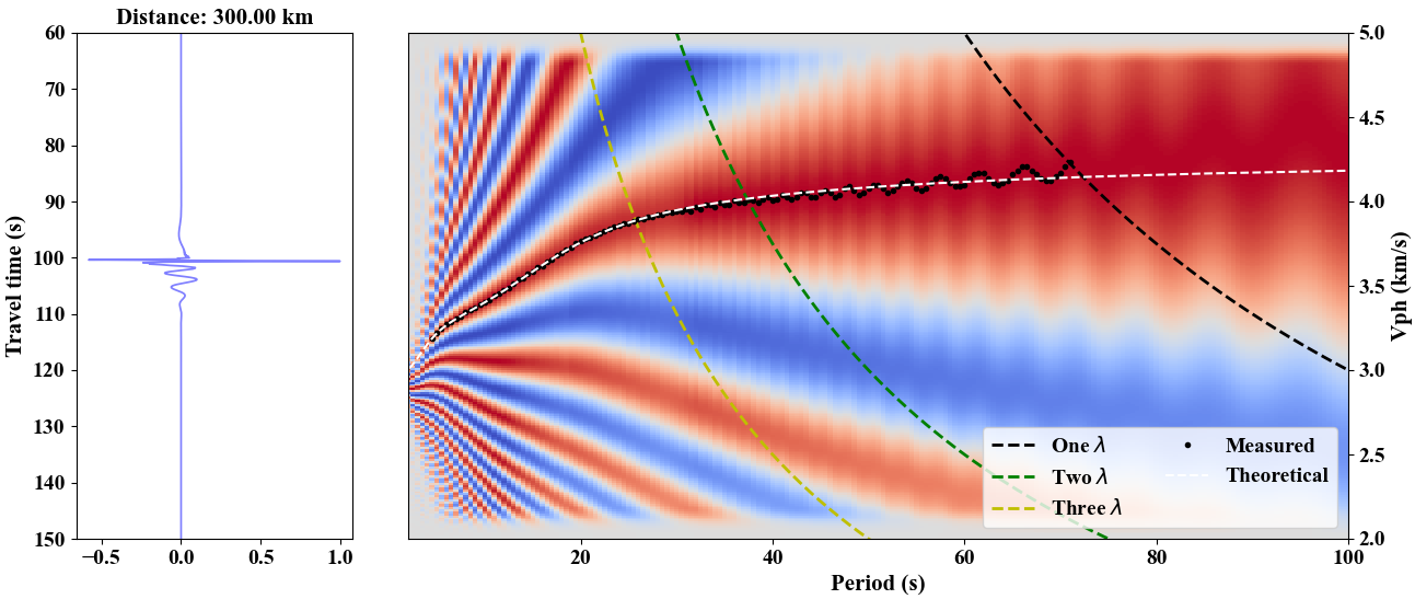
DC One should note that there are 2$\pi$ ambiguities in the phase velocity diagram, and thus careful consideration should be taken into to estimate reliable dispersion curve. The measured dispersion curve (black dots) matches well with the theoretical data (dashed curve) in the above figure.

References

Ekstro¨m, G., G. A. Abers, and S. C. Webb (2009), Determination of surface-wave phase velocities across USArray from noise and Aki’s spectral formulation, Geophys. Res. Lett., 36, L18301, doi:10.1029/2009GL039131.

Levshin, A. L., T. L. Yanovskaya, A. V. Lander, B. G. Bukchin, M. P. Barmin, L. I. Ratnikova, and E. N. Its (1989), Seismic Surface Waves in a Laterally Inhomogeneous Earth, edited by V. I. Keilis-Borok, Kluwer Acad., Norwell, Mass.

Yao, H., R. D. van der Hilst, and M. V. de Hoop (2006), Surface-wave array tomography in SE Tibet from ambient seismic noise and two-station analysis—I. Phase velocity maps, Geophys. J. Int., 166, 732 – 744, doi:710.1111/j.1365-1246X.2006.03028.x