1. Background
Passive dense array surface wave tomography plays a significant role in probing the earth’s interior with
the development of a large number of dense seismic arrays, attracting researchers’ growing interest in
imaging applications in various scales. These array methods, like beamforming and MASW (multichannel analysis
of surface wave) have been widely used to estimate dispersion curves in past several decades. A new array
stacking technique, the frequency-Bessel (F-J) transform, was proposed about five years ago with some main
advantages of extracting dispersion curves of high-resolution and broad frequency band (Wang et al., 2019).
More importantly, this method facilitates the estimation of multimodal dispersion curves for investimating
underground shear wave velocity structure (Wu et al., 2020; Zhan et al., 2020; Li et al., 2021; Chen et al., 2022;
Ma et al., 2022; Zhang et al., 2022; Xi et al., 2021; Zhou & Chen, 2021; Zhou et al., 2023; Feng et al., 2024;
Chen et al., 2024; Wang et al., 2024; Li et al., 2025; Zhang et al., 2025).
Here we introduce the basic principle of this newly proposed array stacking method.
The vertical-vertical (Z-Z) component cross-correlations in frequency domain $C_{ZZ}(\omega, r)$ from ambient seismic noise
is approximately proportional to the imaginary part of the Green’s function $G_{ZZ}(\omega, r)$ between two receivers with
distance of $r$,
$$
C_{ZZ}(\omega,r) \approx A\cdot Im\{G_{ZZ}(\omega, r)\}, \tag{1}
$$
in which, $\omega$ is angular frequency, and $Im\{\cdot\}$ represents imaginary part. Wang et al (2019) defined
the spectrum $I(\omega, k)$ of the F-J transform as
$$
I(\omega, k)=\int_0^{+\infty}C_{ZZ}(\omega, r)J_0(kr)rdr, \tag{2}
$$
where, $J_0$ is the zeroth-order Bessel function of the first kind. For a flat multi-layered medium,
$G_{ZZ}(\omega, r)$ due to an isotropic source is expressed as
$$
G_{ZZ}(\omega, r)=\int_0^{+\infty}g_z(\omega, \kappa)J_0(\kappa r)\kappa d\kappa, \tag{3}
$$
where, $g_z(\omega, k)$ is the kernel function of the medium, and it is inversely proportional to the surface wave
dispersion equation, which means that $g_{z}(\omega, \kappa)$ reaches infinity at roots (dispersion curve) of dispersion equation.
Now we use $(1)$, $(2)$ and $(3)$ to obtain
$$
I(\omega, k)=\int_0^{+\infty}Im\{\int_0^{+\infty}g_z(\omega, \kappa)J_0(\kappa r) \kappa d\kappa\}J_0(kr)rdr. \tag{4}
$$
Note the orthogonality of $J_0$, $\int_0^{+\infty}J_0(kr)rdr\int_0^{+\infty}J_0(\kappa r)\kappa d\kappa=\frac{\delta(k-\kappa)}{k}$,
and thus we have
$$
I(\omega, k) \approx A \cdot Im\{g_z(\omega, k)\}. \tag{5}
$$
$(5)$ shows that $I(\omega, k)$ is infinity at the dispersion point. This is the basic idea that we can estimate dispersion curves
utilizing the F-J transform. For F-J dispersion spectrums showing Love and Rayleigh wave dispersion curves from other components:
Z-R (vertical-Radial), R-Z, T-T (Transverse-Transverse) and R-R (radial-radial), readers can refer to the work by Hu et al. (2020).
3.1 Utilizing the CC-FJpy package to estimate dispersion curves
There is a convenient Python package named CC-FJpy for extracting dispersion curves developed by members from Xiaofei Chen’s team.
We can find this package on this website (https://github.com/ColinLii/CC-FJpy). Here we show the dispersion diagram result computed
using this package. Cross-corrrelation functions are from synthetic ambient noise based on the following source-receiver configuration.
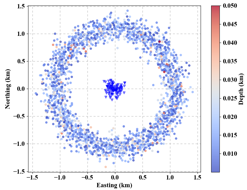
We utilize 100 receivers and 2000 sources to synthesize seismic event. Synthetic ambient noise is generated according to steps
described in this blog. Here we show the dispersion diagram using CC-FJpy.
 1
 2
 3
 4
 5
 6
 7
 8
 9
10
11
12
13
14
15
16
17
18
19
20
21
22
23
24
25
26
27
28
29
30
31
32
33
34
35
36
37
38
39
40
41
42
43
44
45
46
47
48
49
50
51
52
53
54
55
56
57
58
59
60
61
62
63
64
65
66
67
68
69
|
import numpy as np
from obspy import read
import ccfj
import matplotlib.pyplot as plt
from glob import glob

# Match cross-correlation time function files
files = sorted(glob('ccf/*.SAC'))
# Frequency limitations of dispersion diagram
f1 = 0; f2 = 60
# Half time window width of cross-correlations
t0 = 10
t1 = -t0; t2 = t0
dist = []; data = []
ccfr = []; ccfi = []
index = 0
for sac in files:
    tr = read(sac)[0]
	# inster-receiver distance in km is stored in "dist" attribute
    dist.append(tr.stats.sac.dist)
    b = tr.stats.sac.b
    dt = tr.stats.delta
    n1 = int((t1-b)/dt); n2 = int((t2-b)/dt)
    d = tr.data[n1: n2+1]
    d = np.fft.fftshift(d)
    tmp = np.fft.fft(d)
    n = len(tmp)
    tmp = tmp[:n//2]
    ccfr.append(tmp.real)
    index += 1
ccfr = np.array(ccfr)
nd = len(d)
dist = np.array(dist) * 1e3
index = np.argsort(dist)

dist = dist[index]
ccfr = ccfr[index]
# Phase velocity testing range
c1 = 0.25; c2 = 0.75; nc = 501
c = np.linspace(c1*1e3, c2*1e3, nc)
f = np.arange(nd) / dt / (nd-1)
fn1 = int(f1*nd*dt); fn2 = int(f2*nd*dt)
nf = fn2 - fn1 + 1; nr = len(dist)

# Compute dispersion diagram using the F-J transform
im = ccfj.fj_noise(ccfr[:, fn1: fn2+1], dist, c,
                   f[fn1: fn2+1], fstride=1, itype=1,
                   func=0, num=1)
im = np.maximum(im, 0)
# Normalization along the frequancy axis
for i in range(len(im[0])):
    im[:, i] /= abs(im[:, i]).max()
f = f[fn1: fn2+1]
# Load theoretical dispersion curves
dc = np.loadtxt('syn-disp.txt')
dc = dc[::4]
# Visualize dispersion diagram
plt.figure(figsize=(12, 8))
plt.pcolormesh(f, c/1e3, im**2, cmap='jet')
plt.scatter(dc[:, 2], dc[:, 3], marker='o', s=0.5, facecolor='w', alpha=0.5)
plt.plot(f, f*dist.max()/1e3, 'w--')
plt.xlabel('Frequency (Hz)', fontsize=20)
plt.ylabel('Phase velocity (km/s)', fontsize=20)
plt.xlim(f1, f2)
plt.ylim(c1, c2)
plt.xticks(fontsize=17)
plt.yticks(fontsize=17)
plt.tight_layout()
plt.show()
|
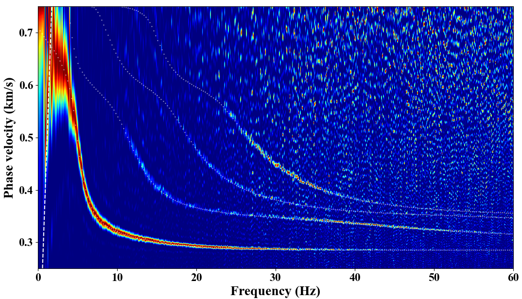 White dots in the above figure are theoretical dispersion curves from the fundamental mode to the third higher mode.
4. Multimodal dispersion curves from field ambient noise
4.1 Field applications: small-scale result from La Réunion Island
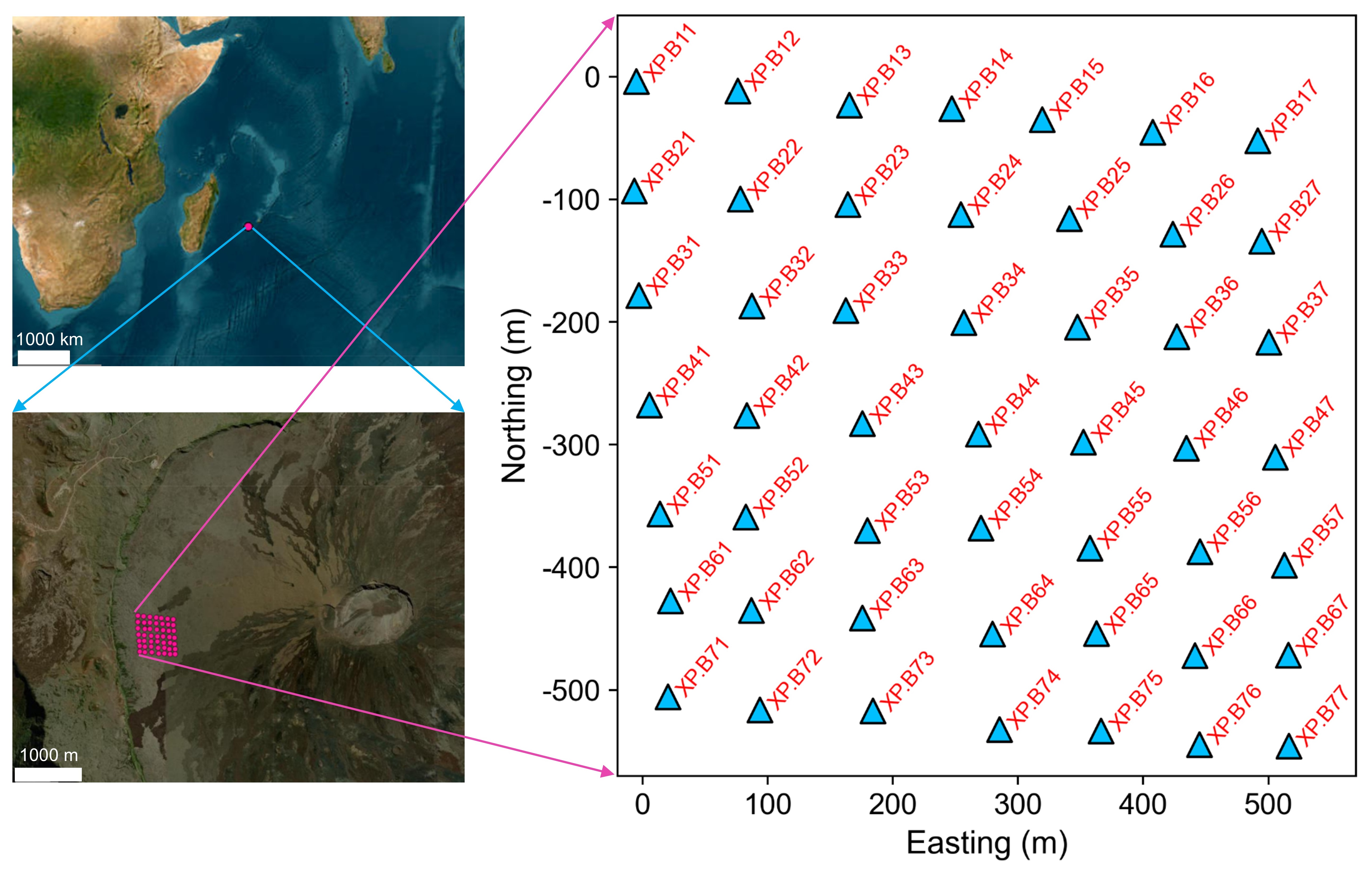
We collected one-hour (2014-07-05T12:00:00-2014-07-05T13:00:00) continuous seismic waveform data of a seismic arrray composed of 49 short period vertical seismic stations deployed on Piton de la Fournaise volcano (La Réunion Island, Indian Ocean, France) for one month. The aperture size of this seismic array is approximately 750 m with station neighboring spacing of ~ 100 m. The continuous waveform data are from the seismic data center RESIF of France, and one can download these seismic data using the Python package Obspy (Examples of downloading seismic data can de found at: https://geophydog.cool/post/python_data_processing/ ). Here is how we request station information about this seismic array: put the link into your browser address bar http://ws.resif.fr/fdsnws/station/1/query?&network=XP&station=B*&channel=DPZ&format=text.
These key parameter settings: network=XP, station=B* and channel=DPZ, can help you find these stations. Push the Enter key and you can get details as below:
 1
 2
 3
 4
 5
 6
 7
 8
 9
10
11
12
13
14
15
16
17
18
19
20
21
22
23
24
25
26
27
28
29
30
31
32
33
34
35
36
37
38
39
40
41
42
43
44
45
46
47
48
49
50
|
#Network|Station|Latitude|Longitude|Elevation|SiteName|StartTime|EndTime
XP|B11|-21.244435|55.682250|2195.1|Piton de la Fournaise, Volcarray antenna B, node 11|2014-07-03T00:00:00|2014-08-01T05:50:00
XP|B12|-21.244502|55.683030|2196.1|Piton de la Fournaise, Volcarray antenna B, node 12|2014-07-03T00:00:00|2014-08-01T05:50:00
XP|B13|-21.244606|55.683890|2197.6|Piton de la Fournaise, Volcarray antenna B, node 13|2014-07-03T00:00:00|2014-08-01T05:50:00
XP|B14|-21.244632|55.684679|2200.6|Piton de la Fournaise, Volcarray antenna B, node 14|2014-07-03T00:00:00|2014-08-01T05:50:00
XP|B15|-21.244713|55.685375|2199.4|Piton de la Fournaise, Volcarray antenna B, node 15|2014-07-03T00:00:00|2014-08-01T05:50:00
XP|B16|-21.244806|55.686227|2201.1|Piton de la Fournaise, Volcarray antenna B, node 16|2014-07-03T00:00:00|2014-08-01T05:50:00
XP|B17|-21.244868|55.687035|2205.7|Piton de la Fournaise, Volcarray antenna B, node 17|2014-07-03T00:00:00|2014-08-01T05:50:00
XP|B21|-21.245241|55.682234|2198.9|Piton de la Fournaise, Volcarray antenna B, node 21|2014-07-03T00:00:00|2014-08-01T05:50:00
XP|B22|-21.245299|55.683052|2199.0|Piton de la Fournaise, Volcarray antenna B, node 22|2014-07-03T00:00:00|2014-08-01T05:50:00
XP|B23|-21.245338|55.683879|2195.8|Piton de la Fournaise, Volcarray antenna B, node 23|2014-07-03T00:00:00|2014-08-01T05:50:00
XP|B24|-21.245409|55.684750|2195.1|Piton de la Fournaise, Volcarray antenna B, node 24|2014-07-03T00:00:00|2014-08-01T05:50:00
XP|B25|-21.245438|55.685584|2197.6|Piton de la Fournaise, Volcarray antenna B, node 25|2014-07-03T00:00:00|2014-08-01T05:50:00
XP|B26|-21.245553|55.686382|2202.8|Piton de la Fournaise, Volcarray antenna B, node 26|2014-07-03T00:00:00|2014-08-01T05:50:00
XP|B27|-21.245603|55.687066|2205.8|Piton de la Fournaise, Volcarray antenna B, node 27|2014-07-03T00:00:00|2014-08-01T05:50:00
XP|B31|-21.246009|55.682270|2196.8|Piton de la Fournaise, Volcarray antenna B, node 31|2014-07-03T00:00:00|2014-08-01T05:50:00
XP|B32|-21.246086|55.683143|2194.9|Piton de la Fournaise, Volcarray antenna B, node 32|2014-07-03T00:00:00|2014-08-01T05:50:00
XP|B33|-21.246118|55.683868|2193.9|Piton de la Fournaise, Volcarray antenna B, node 33|2014-07-03T00:00:00|2014-08-01T05:50:00
XP|B34|-21.246204|55.684776|2192.3|Piton de la Fournaise, Volcarray antenna B, node 34|2014-07-03T00:00:00|2014-08-01T05:50:00
XP|B35|-21.246236|55.685652|2196.5|Piton de la Fournaise, Volcarray antenna B, node 35|2014-07-03T00:00:00|2014-08-01T05:50:00
XP|B36|-21.246304|55.686417|2197.5|Piton de la Fournaise, Volcarray antenna B, node 36|2014-07-03T00:00:00|2014-08-01T05:50:00
XP|B37|-21.246345|55.687124|2202.8|Piton de la Fournaise, Volcarray antenna B, node 37|2014-07-03T00:00:00|2014-08-01T05:50:00
XP|B41|-21.246818|55.682350|2193.6|Piton de la Fournaise, Volcarray antenna B, node 41|2014-07-03T00:00:00|2014-08-01T05:50:00
XP|B42|-21.246892|55.683105|2193.2|Piton de la Fournaise, Volcarray antenna B, node 42|2014-07-03T00:00:00|2014-08-01T05:50:00
XP|B43|-21.246949|55.683996|2189.7|Piton de la Fournaise, Volcarray antenna B, node 43|2014-07-03T00:00:00|2014-08-01T05:50:00
XP|B44|-21.247023|55.684892|2189.9|Piton de la Fournaise, Volcarray antenna B, node 44|2014-07-03T00:00:00|2014-08-01T05:50:00
XP|B45|-21.247081|55.685699|2192.3|Piton de la Fournaise, Volcarray antenna B, node 45|2014-07-03T00:00:00|2014-08-01T05:50:00
XP|B46|-21.247123|55.686494|2195.5|Piton de la Fournaise, Volcarray antenna B, node 46|2014-07-03T00:00:00|2014-08-01T05:50:00
XP|B47|-21.247189|55.687176|2198.9|Piton de la Fournaise, Volcarray antenna B, node 47|2014-07-03T00:00:00|2014-08-01T05:50:00
XP|B51|-21.247618|55.682431|2191.5|Piton de la Fournaise, Volcarray antenna B, node 51|2014-07-03T00:00:00|2014-08-01T05:50:00
XP|B52|-21.247642|55.683097|2191.4|Piton de la Fournaise, Volcarray antenna B, node 52|2014-07-03T00:00:00|2014-08-01T05:50:00
XP|B53|-21.247737|55.684038|2188.8|Piton de la Fournaise, Volcarray antenna B, node 53|2014-07-03T00:00:00|2014-08-01T05:50:00
XP|B54|-21.247717|55.684914|2184.6|Piton de la Fournaise, Volcarray antenna B, node 54|2014-07-03T00:00:00|2014-08-01T05:50:00
XP|B55|-21.247862|55.685753|2188.2|Piton de la Fournaise, Volcarray antenna B, node 55|2014-07-03T00:00:00|2014-08-01T05:50:00
XP|B56|-21.247885|55.686598|2190.4|Piton de la Fournaise, Volcarray antenna B, node 56|2014-07-03T00:00:00|2014-08-01T05:50:00
XP|B57|-21.247984|55.687250|2191.9|Piton de la Fournaise, Volcarray antenna B, node 57|2014-07-03T00:00:00|2014-08-01T05:50:00
XP|B61|-21.248260|55.682514|2187.3|Piton de la Fournaise, Volcarray antenna B, node 61|2014-07-03T00:00:00|2014-08-01T05:50:00
XP|B62|-21.248327|55.683142|2186.3|Piton de la Fournaise, Volcarray antenna B, node 62|2014-07-03T00:00:00|2014-08-01T05:50:00
XP|B63|-21.248382|55.683998|2185.0|Piton de la Fournaise, Volcarray antenna B, node 63|2014-07-03T00:00:00|2014-08-01T05:50:00
XP|B64|-21.248497|55.685004|2181.1|Piton de la Fournaise, Volcarray antenna B, node 64|2014-07-03T00:00:00|2014-08-01T05:50:00
XP|B65|-21.248491|55.685805|2183.6|Piton de la Fournaise, Volcarray antenna B, node 65|2014-07-03T00:00:00|2014-08-01T05:50:00
XP|B66|-21.248650|55.686564|2184.9|Piton de la Fournaise, Volcarray antenna B, node 66|2014-07-03T00:00:00|2014-08-01T05:50:00
XP|B67|-21.248645|55.687283|2188.6|Piton de la Fournaise, Volcarray antenna B, node 67|2014-07-03T00:00:00|2014-08-01T05:50:00
XP|B71|-21.248964|55.682494|2183.6|Piton de la Fournaise, Volcarray antenna B, node 71|2014-07-03T00:00:00|2014-08-01T05:50:00
XP|B72|-21.249059|55.683207|2180.3|Piton de la Fournaise, Volcarray antenna B, node 72|2014-07-03T00:00:00|2014-08-01T05:50:00
XP|B73|-21.249066|55.684079|2180.8|Piton de la Fournaise, Volcarray antenna B, node 73|2014-07-03T00:00:00|2014-08-01T05:50:00
XP|B74|-21.249198|55.685058|2176.3|Piton de la Fournaise, Volcarray antenna B, node 74|2014-07-03T00:00:00|2014-08-01T05:50:00
XP|B75|-21.249208|55.685843|2178.9|Piton de la Fournaise, Volcarray antenna B, node 75|2014-07-03T00:00:00|2014-08-01T05:50:00
XP|B76|-21.249305|55.686599|2181.2|Piton de la Fournaise, Volcarray antenna B, node 76|2014-07-03T00:00:00|2014-08-01T05:50:00
XP|B77|-21.249316|55.687287|2184.2|Piton de la Fournaise, Volcarray antenna B, node 77|2014-07-03T00:00:00|2014-08-01T05:50:00
|
Save above station information in a text file, say ‘XP.lst’ for requesting continuous seismic waveform data. We convert geographic longitudes and latitudes into Cartesian coordinates by setting the longtude and latitude of station XP.B11 as the origin. The following codes show how we perform the conversion dedails.
 1
 2
 3
 4
 5
 6
 7
 8
 9
10
11
12
13
14
15
16
17
18
19
20
21
22
23
24
|
import sys
from geopy.distance import geodesic
from obspy.taup.taup_geo import calc_dist_azi as cda
import numpy as np

x0 = 55.68225
y0 = -21.244435
p0 = (y0, x0)
with open('XP.lst', 'r') as fin:
    lines = fin.readlines()
    out = ''
    for line in lines:
        tmp = line.strip().split()
        x = float(tmp[3]); y = float(tmp[2])
        p1 = (y, x)
        dist = geodesic(p0, p1, ellipsoid='WGS-84').km
        _, az, _ = cda(y0, x0, y, x, 6371, 0)
        az = az * np.pi / 180
        dx = np.sin(az) * dist
        dy = np.cos(az) * dist
        out += ('.'.join(tmp[:2]) + ' %f %f %s\n'%(dx, dy, tmp[4]))

with open('xy.lst', 'w') as fout:
    fout.write(out)
|
The relative Cartesian coordinates of all stations are save in file xy.lst that contains four columns: network.station, easting (km), northing (km) and elevation (m).
Here we give the python codes for retirving seismic data from RESIF data center:
 1
 2
 3
 4
 5
 6
 7
 8
 9
10
11
12
13
14
15
16
17
18
19
20
21
22
23
24
25
26
27
28
29
30
31
32
33
34
35
36
37
38
39
40
41
42
43
44
45
46
47
48
49
50
51
|
from obspy.clients.fdsn.client import Client
from obspy.core import UTCDateTime, Stream
import numpy as np
import os
import sys
from glob import glob

client = Client('RESIF')
t1 = UTCDateTime('2014-07-05T12:00:00')
t2 = UTCDateTime('2014-07-05T13:00:00')
sta = []
with open('XP.lst', 'r') as fin:
    for line in fin.readlines():
        tmp =line.strip().split('|')
        sta.append(tmp[:2])
seg = 1 * 3600
ch = 'DPZ'
print(ch)
tt = t1
while tt < t2:
    dirname = '%s/'%str(tt.date)
    if not os.path.exists(dirname):
        os.mkdir(dirname)
    print(tt)
    hour = '%02d_'%(tt.hour)
    for ns in sta:
        files = glob(dirname+'/'+hour+ns[0]+'.'+ns[1]+'*.SAC')
        if len(files) > 0:
            continue
        try:
            st = client.get_waveforms(network=ns[0], station=ns[1],
                                  channel=ch, location='*',
                                  starttime=tt, endtime=tt+seg)
            stc = Stream()
            for i, tr in enumerate(st):
                if len(tr.data) < 10:
                    continue
                tr.data = -tr.data.mean() + tr.data
                tr.detrend()
                tr.taper(0.001)
                stc.append(tr)
            stc.merge(fill_value=0)
            for tr in stc:
                sac = dirname + hour+ '.'.join([tr.stats.network,
                                           tr.stats.station,
                                           tr.stats.channel,
                                           'SAC'])
                tr.write(sac, format='SAC')
        except Exception:
            print('No data of', ns[0], ns[1])
    tt += seg
|
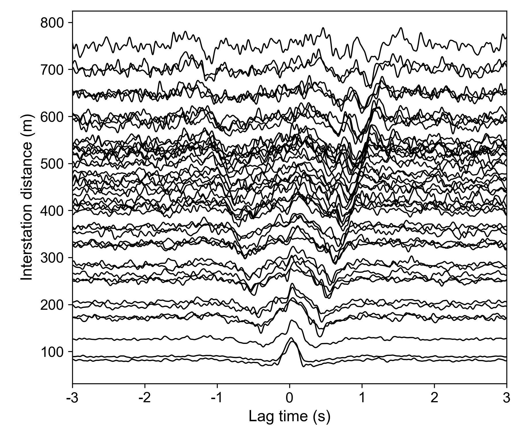
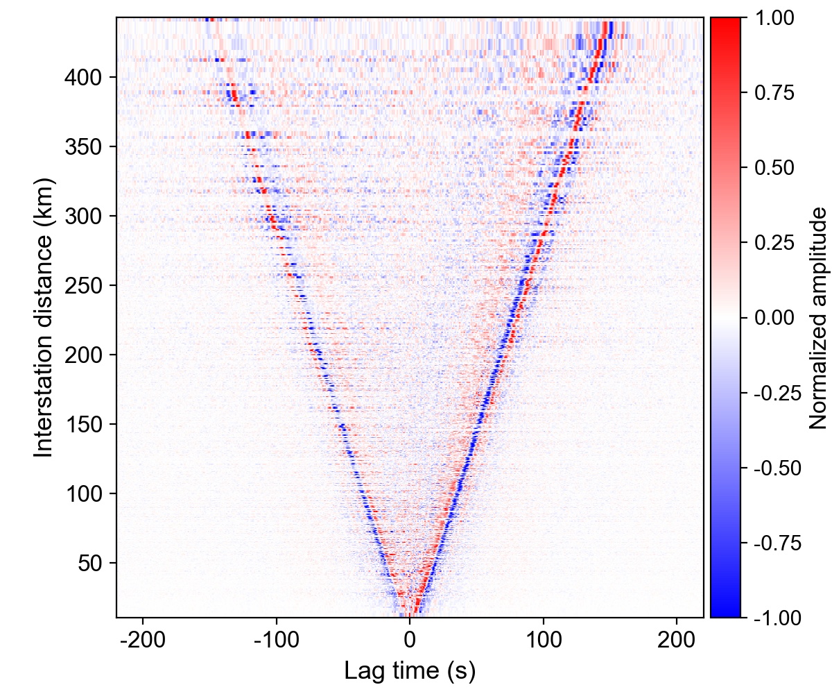
Two-minute raw data segments were splitted for performing pre-processing (removing mean, trend and tapering, normalization in time domain and spectral whitening), and computing cross-correlation functions (CCFs) with an overlap ratio of 50% (one minute). Here we show CCFs (waveforms on the frequency band of 0.5–15 Hz) between station XP.B11 and the other stations. These processing steps follow the details by Bense net al. (2007), generating CCFs of whole station-pairs:
 1
 2
 3
 4
 5
 6
 7
 8
 9
10
11
12
13
14
15
16
17
18
19
20
21
22
23
24
25
26
27
28
29
30
31
32
33
34
35
36
37
38
39
40
41
42
43
44
45
46
47
48
49
50
51
52
53
54
55
56
57
58
59
60
61
62
63
64
65
66
67
68
69
70
71
72
73
74
75
76
77
78
79
80
81
82
83
84
85
86
87
88
89
90
91
92
93
94
95
96
97
98
99
|
import numpy as np
from obspy import read, UTCDateTime
from numpy import ones, convolve
import re
import glob
import os
from obspy.core import Trace, AttribDict
from scipy.signal import hilbert, sosfilt, zpk2sos, sosfilt, iirfilter
from scipy.signal.windows import hann

def process_trace(data, nfft, operator, p=0.01):
    d = data - np.mean(data); n = len(d)
    sn = int(n*p); hn = 2 * sn; h = hann(hn)
    d[:sn] *= h[:sn]; d[-sn:] *= h[-sn:]
    fd = np.fft.fft(d, nfft)
    fd = fd / np.convolve(abs(fd), operator, 'same')
    fd[np.isnan(fd)] = 0
    return fd

sta = {}
with open('xy.lst', 'r') as fin:
    for line in fin.readlines():
        tmp = line.strip().split()
        sta[tmp[0]] = [float(dd) for dd in tmp[1: 3]]
f1 = 0.5; f2 = 50
dt = 0.004; fs = 1 / dt
h = 4; N = 2 * h + 1
operator = np.ones(N) / N
segt = 2 * 60
ot = 1 * 60; pt = segt - ot
segn = int(segt/dt)
pn = int((segt-ot)/dt)
nfft = 2 * int(segt*0.55/dt) + 1
t = np.arange(nfft) * dt - nfft//2*dt
t1 = -60; t2 = 60
tn1 = int((t1-t.min())/dt); tn2 = int((t2-t.min())/dt) + 1
t = t[tn1: tn2]
cor = Trace(t)
cor.stats.delta = dt
cor.stats.sac = AttribDict({})
cor.stats.sac.b = t[0]
cor.data = np.zeros(nfft, dtype=float)

date = '2014-07-05'
hour = 12
print('Read data ...')
try:
    st = read(date+'/%02d_XP.B*Z.SAC'%(hour))
    lm = len(st)
    if lm < 2:
        print('No enough data!!!')
        exit(1)
except Exception:
    pass
ccfdir = 'CCF_%s_%02d/'%(date, hour)
if not os.path.exists(ccfdir):
    os.mkdir(ccfdir)
utc1 = st[0].stats.starttime
utc2 = st[0].stats.endtime
for tr in st:
    if tr.stats.starttime < utc1:
        utc1 = tr.stats.starttime
    if tr.stats.endtime > utc2:
        utc2 = tr.stats.endtime
ln = int((utc2-utc1+segt)/dt)
print('Store data ...')
ns = []; all_data = np.zeros((lm, ln))
for i in range(lm):
    n1 = int((st[i].stats.starttime-utc1)/dt)
    all_data[i, n1: n1+len(st[i].data)] = st[i].data
    ns.append(st[i].stats.network+'.'+st[i].stats.station)
print('Preprocess data ...')
data_fd = []
for i in range(lm):
    dn1 = 0
    tmp = []
    while dn1 <= ln-segn:
        dn2 = dn1 + segn
        fd = process_trace(all_data[i, dn1: dn2], nfft, operator)
        tmp.append(fd)
        dn1 += pn
    data_fd.append(tmp)
print('CCF ...')
nstack = len(data_fd[0])
for si in range(lm-1):
    xi, yi = sta[ns[si]][:2]
    for sj in range(si+1, lm):
        xj, yj = sta[ns[sj]][:2]
        ccfname = 'COR_' + ns[si] +'_' + ns[sj] + '.SAC'
        ccfd = np.zeros(nfft, dtype=complex)
        dist = ( (xi-xj)**2 + (yi-yj)**2 )**0.5
        cor.stats.sac.dist = dist
        for sk in range(nstack):
            ccfd += (data_fd[si][sk]*np.conjugate(data_fd[sj][sk]))
        cor.data = np.fft.ifftshift(np.fft.ifft(ccfd)).real[tn1: tn2]
        cor.stats.sac.evlo = xi; cor.stats.sac.evla = yi
        cor.stats.sac.stlo = xj; cor.stats.sac.stla = yj
        cor.filter('bandpass', freqmin=f1, freqmax=f2, corners=4, zerophase=True)
        cor.write(ccfdir+ccfname)
|
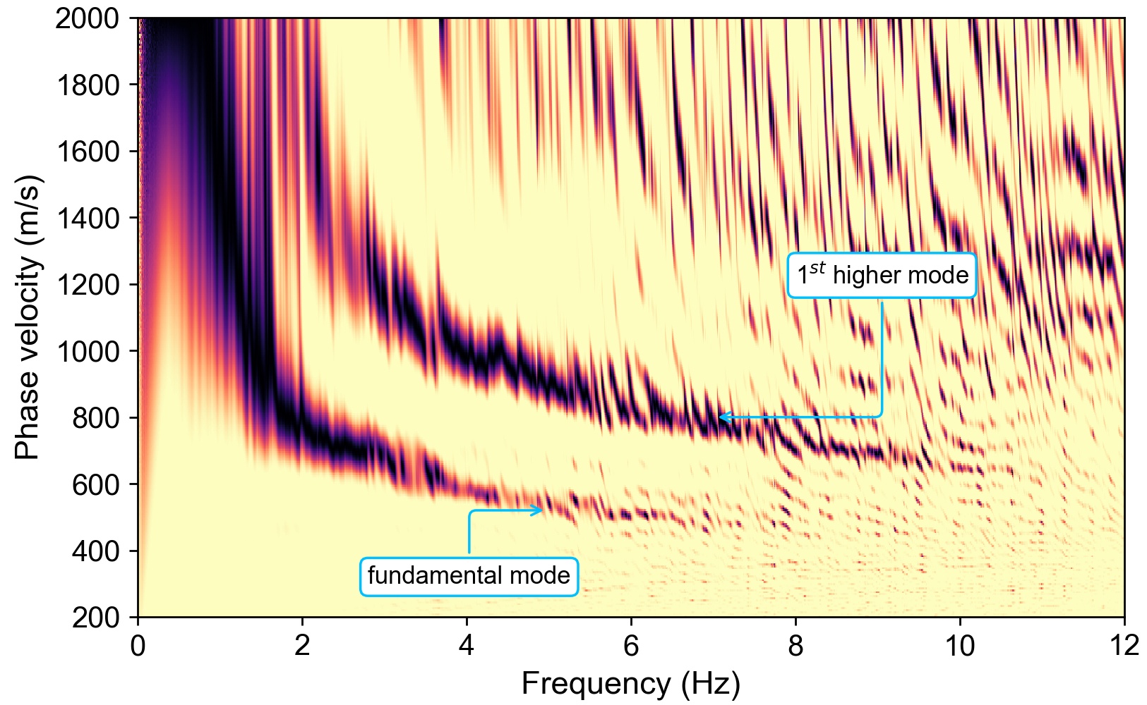
Now we compute the Rayleigh wave dispersion diagram using the F-J transform from CCFs of the all station-pairs in this whole array. Two surface wave modes emerge from the F-J dspectrum, showing the fundamental-mode and the first higher-mode dispersion curves. Tip: the F-J dispersion diagram can be obtained utilizing the CC-FJpy Python package ( https://github.com/ColinLii/CC-FJpy ).
 1
 2
 3
 4
 5
 6
 7
 8
 9
10
11
12
13
14
15
16
17
18
19
20
21
22
23
24
25
26
27
28
29
30
31
32
33
34
35
36
37
38
39
40
41
42
43
44
45
46
47
48
49
50
51
52
53
54
55
56
57
58
59
60
61
62
63
64
65
66
67
68
69
70
71
72
|
import numpy as np
from obspy import read
import ccfj
import matplotlib.pyplot as plt
from glob import glob
import os

ccf_dir = 'CCF_2014-07-05_12'
tag = 'XP.B*'
files = sorted(glob(ccf_dir+'/COR_%s_%s.SAC'%(tag, tag)))
f1 = 0; f2 = 12
t0 = 60; t1 = -t0; t2 = t0
dist = []; ccfr = []
for sac in files:
    tr = read(sac)[0]
    y1 = tr.stats.sac.evla; x1 = tr.stats.sac.evlo
    y2 = tr.stats.sac.stla; x2 = tr.stats.sac.stlo
    gcarc = ( (x1-x2)**2 + (y1-y2)**2 ) ** 0.5 * 1e3
    if gcarc < 1e-6:
        continue
    dist.append(gcarc)
    b = tr.stats.sac.b
    dt = tr.stats.delta
    n1 = int((t1-b)/dt); n2 = int((t2-b)/dt)
    d = tr.data[n1: n2+1]
    d = np.fft.fftshift(d)
    tmp = np.fft.fft(d)
    n = len(tmp)
    ccfr.append(tmp.real[:n//2])

print('CCF files:', len(files))
ccfr = np.array(ccfr)
nd = len(d)
dist = np.array(dist)
index = np.argsort(dist)
dist = dist[index]
ccfr = ccfr[index]

print('rmin: %.6f m rmax: %.6f m'%(dist.min(), dist.max()))
c1 = 200; c2 = 2000; nc = 301
c = np.linspace(c1, c2, nc)
f = np.arange(nd) / dt / (nd-1)
fn1 = int(f1*nd*dt); fn2 = int(f2*nd*dt)
nf = fn2 - fn1 + 1; nr = len(dist)

im = ccfj.fj_noise(ccfr[:, fn1: fn2+1], dist, c,
                   f[fn1: fn2+1], fstride=1, itype=1,
                   func=1, num=1)
im[im<=0] = 0
for i in range(len(im[0])):
    if im[:, i].max() < 1e-8:
        continue
    im[:, i] /= np.abs(im[:, i]).max()
im = im**2

arrowprops = dict(
    arrowstyle='->',
    connectionstyle='angle,angleA=90,angleB=0,rad=10',
    color='#00BFFF')
bbox = dict(boxstyle='round', fc='w', color='#00BFFF')
fig = plt.figure(figsize=(6.5, 4))
fig.subplots_adjust(bottom=0.125, right=0.98, top=0.975, left=0.12)
ax = plt.subplot(111)
ax.tick_params(labelsize=12)
im = ax.pcolormesh(f, c, fj, cmap='magma_r')
ax.annotate('fundamental mode', xytext=(2.8, 300), xy=(5, 520),
            arrowprops=arrowprops, bbox=bbox)
ax.annotate('1$^{st}$ higher mode', xytext=(8, 1200), xy=(7, 800),
            arrowprops=arrowprops, bbox=bbox)
ax.set_xlabel('Frequency (Hz)', fontsize=13)
ax.set_ylabel('Phase velocity (m/s)', fontsize=13)
plt.show()
|
4.2 Field applications: crustal and uppermost mantle-scale result of northwestern United States
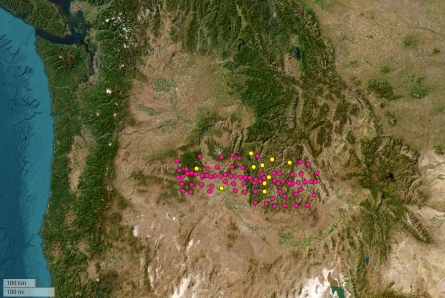
86 broadband seismic stations had been installed in the northwestern US between 2011 and 2013.
We collocted vertical contunuous seismic recordings made by 76 seismic stations (red solid circles) while 10 stations (yellow solid circles) failed
in recording data in January, 2012. This seismic array have an aperture of ~ 450 km with a spacing of ~ 50 km.
Daily seismic recordings of all stations are sotred in corresponding date directory.
We splitted daily seismic data in one-hour segments for performing pre-processing, removing mean, trend, tapering,
and spectral whitening included, and applied an overlap of 50% (30 minutes) to process next one-hour raw data.
Finally, surface waves of high signal-to-noise ratios emerge from stacked hourly cross-correlation functions.
Compute ambient noise cross-correlations with command python overlap_ccf.py 2012-01 Z Z XT.lst, where overlap_ccf.py
contains the folowing Python codes. These codes with match all daily directories of January, 2012 with 2012-01, and Z denote vertical
component. There are at least four columns in file XT.lst: network|station|latitude|longitude, saying XT|D01|43.635601|-113.740097 …
  1
  2
  3
  4
  5
  6
  7
  8
  9
 10
 11
 12
 13
 14
 15
 16
 17
 18
 19
 20
 21
 22
 23
 24
 25
 26
 27
 28
 29
 30
 31
 32
 33
 34
 35
 36
 37
 38
 39
 40
 41
 42
 43
 44
 45
 46
 47
 48
 49
 50
 51
 52
 53
 54
 55
 56
 57
 58
 59
 60
 61
 62
 63
 64
 65
 66
 67
 68
 69
 70
 71
 72
 73
 74
 75
 76
 77
 78
 79
 80
 81
 82
 83
 84
 85
 86
 87
 88
 89
 90
 91
 92
 93
 94
 95
 96
 97
 98
 99
100
101
102
103
104
105
106
107
108
109
110
111
112
113
114
115
116
117
118
119
120
121
122
123
124
125
126
127
128
129
130
131
|
import numpy as np
from obspy import read
from numpy import ones, convolve
import re
import glob
import os
from obspy.core import Trace, AttribDict
import sys
from scipy.signal import hilbert
from scipy.signal.windows import hann

def process_trace(data, nfft, operator, p=0.01):
    d = data - np.mean(data); n = len(d)
    sn = int(n*p); hn = 2 * sn; h = hann(hn)
    d[:sn] *= h[:sn]; d[-sn:] *= h[-sn:]
    fd = np.fft.fft(d, nfft)
    fd /= np.convolve(np.abs(fd), operator, 'same')
    fd[np.isnan(np.abs(fd))] = 0
    return fd

argc = len(sys.argv)
if argc != 5:
    print('Usage: python %s yyyy-mm-dd channel1 channel2 sta.lst'%sys.argv[0])
    exit(1)

sta = {}
with open(sys.argv[4], 'r') as fin:
    for line in fin.readlines():
        tmp = line.strip().split('|')
        k = tmp[0] + '.' + tmp[1]
        sta[k] = [float(tmp[3]), float(tmp[2])]
f1 = 0.005; f2 = 1
dt = 0.2; fs = 1 / dt
h = 15; N = 2 * h + 1
operator = np.ones(N) / N
segt = 1 * 60 * 60
ot = segt * 0.5; pt = segt - ot
segn = int(segt/dt)
pn = int((segt-ot)/dt)
nfft = 2 * int(0.6*segt/dt) + 1
t = np.arange(nfft) * dt - nfft//2*dt
ct1 = -1500; ct2 = 1500
cn1 = np.argmin(np.abs(ct1-t))
cn2 = np.argmin(np.abs(ct2-t))
t = t[cn1: cn2+1]
cor = Trace(t)
cor.stats.delta = dt
cor.stats.sac = AttribDict({})
cor.stats.sac.b = t[0]

ch1 = sys.argv[2]
ch2 = sys.argv[3]
dirs = sorted(glob.glob(sys.argv[1]+'*'))
for dd in dirs:
    print(dd)
    if dd[-1] != '/':
        dd += '/'
    try:
        st1 = read('%s/*H%s.SAC'%(dd, ch1))
        if ch2 == ch1:
            st2 = st1.copy()
        else:
            st2 = read('%s/*H%s.SAC'%(dd, ch2))
        sta1 = [tr.stats.station for tr in st1]
        sta2 = [tr.stats.station for tr in st2]
        st = []
        for s in sta1:
            if s in sta2:
                st.append([st1[sta1.index(s)], st2[sta2.index(s)]])
        lm = len(st)
        if lm < 2:
            continue
        utc1 = st[0][0].stats.starttime
        utc2 = st[0][0].stats.endtime
        date = '%s'%(str(utc1.date))
        for i in range(len(st)):
            tt11 = st[i][0].stats.starttime
            tt21 = st[i][1].stats.starttime
            tt12 = st[i][0].stats.endtime
            tt22 = st[i][1].stats.endtime
            if utc1 > tt11:
                utc1 = tt11
            if utc1 > tt21:
                utc1 = tt21
            if utc2 < tt12:
                utc2 = tt12
            if utc2 < tt22:
                utc2 = tt22
    except Exception:
        continue
    ccfdir = '%s%s_CCF_%s'%(ch1, ch2, date)
    if not os.path.exists(ccfdir):
        os.mkdir(ccfdir)
    nn = int((utc2-utc1)/dt) + 100
    data1 = np.zeros((lm, nn))
    data2 = np.zeros((lm, nn))
    ns = []; xy = []
    for i in range(lm):
        nb1 = int((st[i][0].stats.starttime-utc1)/dt)
        data1[i, nb1:nb1+len(st[i][0].data)] = st[i][0].data
        nb2 = int((st[i][1].stats.starttime-utc1)/dt)
        data2[i, nb2:nb2+len(st[i][1].data)] = st[i][1].data
        k = st[i][0].stats.network+'.'+st[i][0].stats.station
        ns.append(k)
        xy.append(sta[k])
    data_fd1 = []; data_fd2 = []
    for i in range(lm):
        dn1 = 0
        tmp1 = []; tmp2 = []
        while dn1 <= nn-segn:
            dn2 = dn1 + segn
            fd1 = process_trace(data1[i, dn1: dn2], nfft, operator)
            fd2 = process_trace(data2[i, dn1: dn2], nfft, operator)
            tmp1.append(fd1)
            tmp2.append(fd2)
            dn1 += pn
        data_fd1.append(tmp1); data_fd2.append(tmp2)
    nstack = len(data_fd1[0])
    for si in range(lm-1):
        for sj in range(si+1, lm):
            ccfname = 'COR_' + ns[si] +'_' + ns[sj] + '.SAC'
            ccfd = np.zeros(nfft, dtype=complex)
            for sk in range(nstack):
                ccfd += (data_fd1[si][sk]*np.conjugate(data_fd2[sj][sk]))
            cor.data = np.fft.ifftshift(np.fft.ifft(ccfd)).real[cn1: cn2+1]
            cor.filter('bandpass', freqmin=f1, freqmax=f2, corners=4, zerophase=True)
            cor.stats.sac.evlo = xy[si][0]
            cor.stats.sac.evla = xy[si][1]
            cor.stats.sac.stlo = xy[sj][0]
            cor.stats.sac.stla = xy[sj][1]
            cor.write(ccfdir+'/'+ccfname)
|
Now we compue the F-J dispersion diagram using the following codes:
 1
 2
 3
 4
 5
 6
 7
 8
 9
10
11
12
13
14
15
16
17
18
19
20
21
22
23
24
25
26
27
28
29
30
31
32
33
34
35
36
37
38
39
40
41
42
43
44
45
46
47
48
49
50
51
52
53
54
55
56
57
58
59
60
61
62
63
64
65
|
import numpy as np
from obspy import read
from geopy.distance import geodesic
import ccfj
from glob import glob
from scipy.signal import savgol_filter as sgolay


files = sorted(glob('stack/COR*.SAC'))
f1 = 0; f2 = 0.6
t0 = 1000
t1 = -t0; t2 = t0
print(t1, t2)
dist = []; ccfr = []
index = 0
for sac in files:
    tr = read(sac)[0]
    x1, y1 = tr.stats.sac.stlo, tr.stats.sac.stla
    x2, y2 = tr.stats.sac.evlo, tr.stats.sac.evla
    r = geodesic((y1, x1), (y2, x2), ellipsoid='WGS-84').km
    dist.append(r)
    b = tr.stats.sac.b
    dt = tr.stats.delta
    n1 = int((t1-b)/dt); n2 = int((t2-b)/dt)
    d = tr.data[n1: n2+1]
    d = np.fft.fftshift(d)
    tmp = np.fft.fft(d).real
    n = len(tmp)
    tmp = tmp[:n//2]
    ccfr.append(tmp.real)
    index += 1

print('CCF files:', index)
ccfr = np.array(ccfr)
nd = len(d)
dist = np.array(dist) * 1e3
index = np.argsort(dist)
dist = dist[index]
ccfr = ccfr[index]
for i in range(ccfr.shape[0]):
    ccfr[i] = sgolay(ccfr[i], 11, 2)
for i in range(ccfr.shape[1]):
    ccfr[:, i] = sgolay(ccfr[:, i], 5, 2)

print('Max distance:', dist.max())
c1 = 2500; c2 = 5000; nc = 501
c = np.linspace(c1, c2, nc)
f = np.arange(nd) / dt / (nd-1)
fs = 1 / dt
f = np.arange(nd) * fs / (nd-1)
fn1 = np.argmin(np.abs(f1-f))
fn2 = np.argmin(np.abs(f2-f))

im = ccfj.fj_noise(ccfr[:, fn1: fn2+1], dist, c,
                   f[fn1: fn2+1], fstride=1, itype=1,
                   func=1, num=1)

im[im<0] = 0
for i in range(len(im[0])):
    if im[:, i].max() < 1e-8:
        continue
    im[:, i] /= np.abs(im[:, i]).max()
f = f[fn1: fn2+1]

np.savetxt('fj_XT.txt', im**2)
|
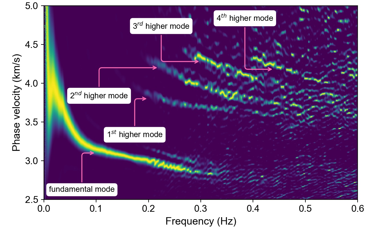
We observed Rayleigh wave dispersion curves of five modes: from the fundamental mode to the fourth higher mode.
 1
 2
 3
 4
 5
 6
 7
 8
 9
10
11
12
13
14
15
16
17
18
19
20
21
22
23
24
25
26
27
28
29
30
|
import numpy as np
import matplotlib.pyplot as plt

fj = np.loadtxt('fj_XT.txt')
nc, nf = fj.shape
f = np.linspace(0, 0.6, nf); c = np.linspace(2500, 5000, nc)

arrowprops = dict(
    arrowstyle='->',
    connectionstyle='angle,angleA=90,angleB=0,rad=10',
    color='#FF69B4', lw=1.25)
bbox = dict(boxstyle='round', fc='w', color='w')
fig = plt.figure(figsize=(6.4, 4))
fig.subplots_adjust(bottom=0.125, right=0.98, top=0.975, left=0.12)
ax = plt.subplot(111)
ax.tick_params(labelsize=12)
im = ax.pcolormesh(f, c/1e3, fj, cmap='viridis')
ax.annotate('fundamental mode', xytext=(0.01, 2.6), xy=(0.1, 3.1),
            arrowprops=arrowprops, bbox=bbox)
ax.annotate('1$^{st}$ higher mode', xytext=(0.12, 3.3), xy=(0.2, 3.8),
            arrowprops=arrowprops, bbox=bbox)
ax.annotate('2$^{nd}$ higher mode', xytext=(0.05, 3.8), xy=(0.22, 4.2),
            arrowprops=arrowprops, bbox=bbox)
ax.annotate('3$^{rd}$ higher mode', xytext=(0.17, 4.7), xy=(0.3, 4.28),
            arrowprops=arrowprops, bbox=bbox)
ax.annotate('4$^{th}$ higher mode', xytext=(0.33, 4.8), xy=(0.44, 4.18),
            arrowprops=arrowprops, bbox=bbox)
ax.set_xlabel('Frequency (Hz)', fontsize=13)
ax.set_ylabel('Phase velocity (km/s)', fontsize=13)
plt.show()
|
References
Bensen, G.D., Ritzwoller, M.H., Barmin, M.P., Levshin, A.L., Lin, F., Moschetti, M.P., Shapiro, N.M. and Yang, Y. (2007), Processing seismic ambient noise data to obtain reliable broad-band surface wave dispersion measurements. Geophysical Journal International, 169: 1239-1260.
Chen, J., Pan, L., Li, Z., & Chen, X. (2022). Continental reworking in the eastern South China Block and its adjacent areas revealed by F-J multimodal ambient noise tomography. Journal of Geophysical Research: Solid Earth, 127, e2022JB024776.
Chen, J., Li, Z., & Chen, X. (2024). A mid-crustal channel of positive radial anisotropy beneath the eastern South China Block from F-J multimodal ambient noise tomography. Geophysical Research Letters, 51, e2024GL110766.
Feng, X., Xia, Y. & Chen, X. (2024). Frequency-Bessel multi-mode surface wave tomography utilizing microseisms excited by energetic typhoons. Sci. China Earth Sci. 67, 3436–3447.
Hu, S., Luo, S., & Yao, H. (2020). The Frequency-Bessel Spectrograms of multicomponent cross-correlation functions from seismic ambient noise. Journal of Geophysical Research: Solid Earth, 125, e2020JB019630.
Li Haiyan, Juqing Chen, Zhengbo Li, Xiaofei Chen, Huiteng Cai, Xuping Feng, Gongheng Zhang, Zhen Jin. (2025). Mid-crustal low-velocity zones beneath Southeastern Coastal China revealed by multimodal ambient noise tomography: Insights into Mesozoic magmatic activities. Tectonophysics, 898, 230636.
Li Z., Jie Zhou, Gaoxiong Wu, Jiannan Wang, Gongheng Zhang, Sheng Dong, Lei Pan, Zhentao Yang, Lina Gao, Qingbo Ma, Hengxin Ren, Xiaofei Chen; CC‐FJpy: A Python Package for Extracting Overtone Surface‐Wave Dispersion from Seismic Ambient‐Noise Cross Correlation. Seismological Research Letters 2021;; 92 (5): 3179–3186.
Ma Q, Pan L, Wang J-, Yang Z and Chen X (2022) Crustal S-Wave Velocity Structure Beneath the Northwestern Bohemian Massif, Central Europe, Revealed by the Inversion of Multimodal Ambient Noise Dispersion Curves. Front. Earth Sci. 10:838751.
Pan Lei, Xiaofei Chen, Jiannan Wang, Zhentao Yang, Dazhou Zhang, Sensitivity analysis of dispersion curves of Rayleigh waves with fundamental and higher modes, Geophysical Journal International, Volume 216, Issue 2, February 2019, Pages 1276–1303
Wang, J., Wu, G., & Chen, X. (2019). Frequency‐Bessel transform method for effective imaging of higher‐mode Rayleigh dispersion curves from ambient seismic noise data. Journal of Geophysical Research: Solid Earth, 124(4), 3708-3723.
Wang P., Chen J., Feng X., Pan L., & Chen X. (2024) Crust and upper mantle S wave velocity structure in eastern Turkey based on ambient noise tomography. Tectonophysics,876, 230267.
Wu, G.-x., Pan, L., Wang, J.-n., & Chen, X. (2020). Shear velocity inversion using multimodal dispersion curves from ambient seismic noise data of USArray transportable array. Journal of Geophysical Research: Solid Earth, 125, e2019JB018213.
Xi Chaoqiang, Jianghai Xia, Binbin Mi, Tianyu Dai, Ya Liu, Ling Ning. (2021). Modified frequency–Bessel transform method for dispersion imaging of Rayleigh waves from ambient seismic noise. Geophysical Journal International, 255(2), 1271–1280.
Zhan Wang, Lei Pan, Xiaofei Chen. (2020) A widespread mid-crustal low-velocity layer beneath Northeast China revealed by the multimodal inversion of Rayleigh waves from ambient seismic noise. Journal of Asian Earth Sciences, 196, 104372.
Zhang S, Zhang G, Feng X, Li Z, Pan L, Wang J and Chen X. (2022). A crustal LVZ in Iceland revealed by ambient noise multimodal surface wave tomography. Front. Earth Sci. 10:1008354.
Zhang Sen, Juqing Chen, Lei Pan, Zhengbo Li, Xiaofei Chen. (2024). Seismic structure of Iceland revealed by ambient noise Rayleigh wave tomography. Tectonophysics, 891, 230511.
Zhang, Yanyan & Chen, Xiaofei & Chen, Juqing & Zhang, Gongheng & Li, Zhengbo & Pan, Lei & Wang, Jiannan & Ding, Zhifeng & Wang, Xingchen & Yuan, Songyong. (2025). Seismic evidence of subduction during the assembly of the North China Craton from multimodal dispersion inversion. Tectonophysics. 904. 230715.
Zhou Jie, & Chen Xiaofei. (2021) Removal of Crossed Artifacts from Multimodal Dispersion Curves with Modified Frequency–Bessel Method. Bulletin of the Seismological Society of America, 112 (1): 143–152.
Zhou, J., Li, Z., & Chen, X. (2023). Extending the frequency band of surface-wave dispersion curves by combining ambient noise and earthquake data and self-adaptive normalization. Journal of Geophysical Research: Solid Earth, 128, e2022JB026040.
 times read