1 Basic principles
In the previous blog Cross Spectral Beamforming, we’ve briefly introduced the basic principles of coherent signal detection with seismic array method beamforming. Here, we will use the cross spectral beamforming in ambient seismic noise cross-correlation functions (NCF). We first show the slowness and back-azimuth detection of Rayleigh waves, and then distant body waves detection will be conducted.
2 Rayleigh waves in NCF
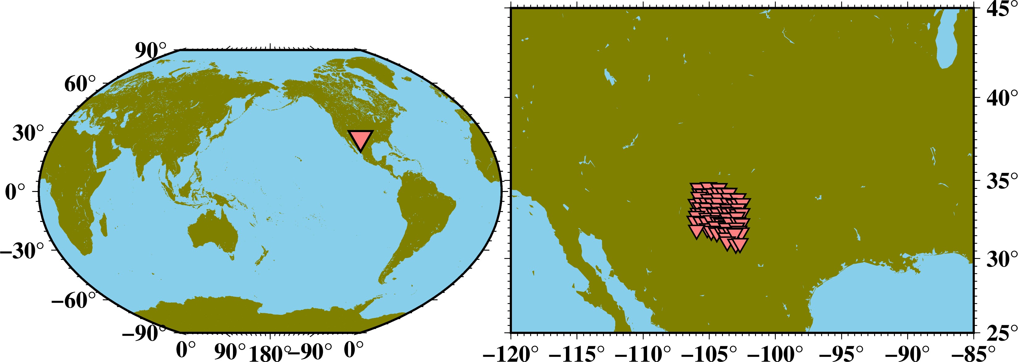
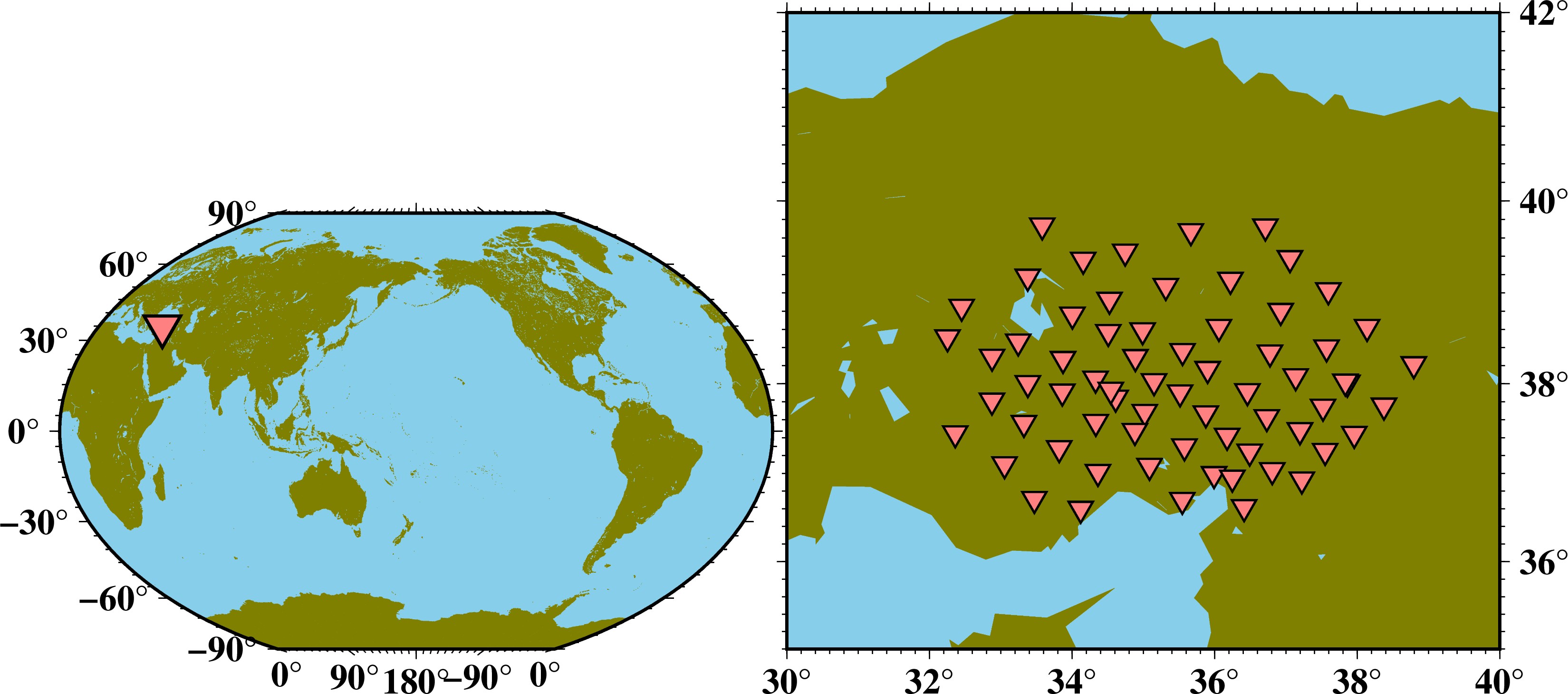
We collect one-month vertical component (here $BHZ$)seismic data in Aug. 2008 recorded by a seismic array named $XR$ installed in the USA. We closely follow the NCF processing steps suggested by Bensen et al. (2007) to compute the one-hour cross-correlations and temporal stacking to obtain the final NCF.
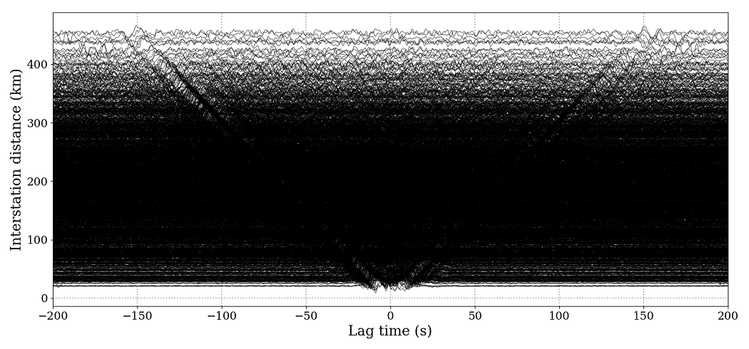
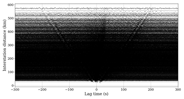
The final NCF waveforms of array $XR$ are shown below, and we can see that the velocity is about $3 \ km/s$ of the coherent signals in the NCF interstation-lag time arrangement.
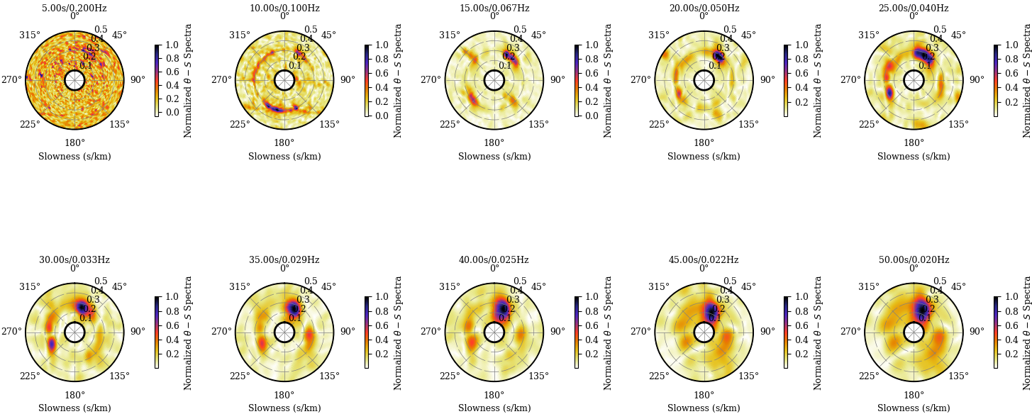
We cut the NCF waveforms in the lag time window of -200 $-$ 200 $s$ to analysis the slowness and back-azimuth of Rayleigh waves.
We suppose that one has installed these Python packages:
numpy , matplotlib, scipy, obspy and geopy.
2.1 Single-frequency analysis
One can find the proper way of estimating a narrow band signal when considering the near frequencies (which differ by $\pm 10 \%$ from the center frequency, Gal et al., 2014; Nakata et al., 2019). Here, we just show the results of single frequency value.
 1
 2
 3
 4
 5
 6
 7
 8
 9
10
11
12
13
14
15
16
17
18
19
20
21
22
23
24
25
26
27
28
29
30
31
32
33
34
35
36
37
38
39
40
41
42
43
44
45
46
47
48
49
50
51
52
53
54
55
56
57
58
59
60
61
62
63
64
65
66
67
68
69
70
71
72
73
74
75
76
77
|
import numpy as np
import matplotlib.pyplot as plt
import matplotlib as mpl
from scipy import fft
from obspy import read
from scipy import interpolate
from geopy.distance import geodesic
from obspy.taup.taup_geo import calc_dist_azi as cda

# Read in NCF files.
st = read('COR*.SAC')


# Obtain the cross-spectra (Fourier spectra of NCF)
ccf = []
pos = []
t0 = 200
t1 = -t0; t2 = t0
for tr in st:
    x1 = tr.stats.sac.evlo; y1 = tr.stats.sac.evla
    x2 = tr.stats.sac.stlo; y2 = tr.stats.sac.stla
    _, az, _ = cda(y1, x1, y2, x2, 6371, 0)
    az = az / 180 * np.pi
    dist = geodesic((y1, x1), (y2, x2), ellipsoid='WGS-84').km
    b = tr.stats.sac.b; dt = tr.stats.delta
    n1 = int((t1-b)/dt); n2 = int((t2-b)/dt)
    d = tr.data[n1: n2+1]; n = len(d)
    fd = np.fft.fft(np.fft.fftshift(d))
    ccf.append(fd); pos.append([np.sin(az)*dist, np.cos(az)*dist])
ccf = np.array(ccf); pos = np.array(pos) * 1e3


## Cross-spectral beamforming analysis.
nf = len(ccf[0])
fs = 1 / dt
# Range of slowness in s/m.
s1 = 1e-4; s2 = 5e-4
sn = 51; bn = 121
slow = np.linspace(s1, s2, sn)
# Range of bazk-azimuth in degree.
baz = np.radians(np.linspace(0, 360, bn))
# Period range.
T = np.linspace(5, 50, 10)
# Scan and plot the spectra of every period/frequency.
plt.figure(figsize=(15, 8))
for ti, tt in enumerate(T):
    ff = 1 / tt; w = 2 * np.pi * ff
    print('Scaning period:', tt, 's ...')
    fn = int(ff*nf/fs)
    P1 = np.zeros((sn, bn), dtype=complex)
    tmp = -1j * w
    for i, ss in enumerate(slow):
        for j, bb in enumerate(baz):
            shift = ss * (-np.sin(bb)*pos[:, 0] - np.cos(bb)*pos[:, 1])
            P1[i, j] = np.dot(ccf[:, fn], np.exp(tmp*shift))
    PP = abs(P1)
    bazz2 = np.linspace(baz[0], baz[-1], 241)
    sloww2 = np.linspace(slow[0], slow[-1], 201)
    inp = interpolate.interp2d(baz, slow, PP, kind='cubic')
    PP = inp(bazz2, sloww2)
    PP = PP / PP.max()
    ax1 = plt.subplot(2, 5, ti+1, projection='polar')
    plt.pcolormesh(bazz2, sloww2*1e3, PP, cmap='CMRmap_r')
    cbar = plt.colorbar(shrink=0.25, pad=0.2)
    cbar.set_label(r'Normalized $\theta-S$ Spectra', fontsize=9)
    cbar.ax.tick_params(labelsize=9)
    ax1.grid(color='gray', ls=(2, (30, 5)), lw=0.5)
    ax1.tick_params(axis='y', colors='k', labelsize=9)
    ax1.set_theta_zero_location('N')
    ax1.set_theta_direction(-1)
    ax1.plot(baz, np.ones(len(baz))*slow.min()*1e3, c='k', lw=2)
    ax1.plot(baz, np.ones(len(baz))*slow.max()*1e3, c='k', lw=2)
    ax1.set_xlabel('Slowness (s/km)', fontsize=9)
    plt.xticks(fontsize=9); plt.yticks(fontsize=9)
    plt.title('%.2fs/%.3fHz'%(tt,1/tt), fontsize=9, pad=15)
plt.tight_layout()
plt.show()
|
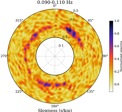
2.2 Extension to Broadband Data Analysis
We just compute the sum of all spectra of every single frequency to obtain the FK beamforming spectra on the given frequency band. Here we show the results when the frequency band is given and we set the frequency band as 0.09$-$ 0.11 $Hz$ and the spectra can be obtained by
 1
 2
 3
 4
 5
 6
 7
 8
 9
10
11
12
13
14
15
16
17
18
19
20
21
22
23
24
25
26
27
28
29
30
31
32
33
34
35
36
37
38
39
40
41
42
43
44
45
46
47
48
49
50
51
52
53
54
55
56
57
58
59
60
61
62
63
64
65
66
67
68
69
70
71
72
73
74
75
76
77
78
|
import numpy as np
import matplotlib.pyplot as plt
import matplotlib as mpl
from scipy import fft
from obspy import read
from scipy import interpolate
from geopy.distance import geodesic
from obspy.taup.taup_geo import calc_dist_azi as cda

# Read in NCF files.
st = read('COR*.SAC')

# Cross spectra.
ccf = []
pos = []
t0 = 200
t1 = -t0; t2 = t0
for tr in st:
    x1 = tr.stats.sac.evlo; y1 = tr.stats.sac.evla
    x2 = tr.stats.sac.stlo; y2 = tr.stats.sac.stla
    _, az, _ = cda(y1, x1, y2, x2, 6371, 0)
    az = az / 180 * np.pi
    dist = geodesic((y1, x1), (y2, x2), ellipsoid='WGS-84').km
    b = tr.stats.sac.b; dt = tr.stats.delta
    n1 = int((t1-b)/dt); n2 = int((t2-b)/dt)
    d = tr.data[n1: n2+1]; n = len(d)
    fd = np.fft.fft(np.fft.fftshift(d))
    ccf.append(fd); pos.append([np.sin(az)*dist, np.cos(az)*dist])
ccf = np.array(ccf); pos = np.array(pos) * 1e3

# Parameter settings.
nf = len(ccf[0])
fs = 1 / dt
s1 = 2e-4; s2 = 5e-4
sn = 51; bn = 121
slow = np.linspace(s1, s2, sn)
baz = np.radians(np.linspace(0, 360, bn))

f = np.arange(nf) * fs / (nf-1)
f1 = 0.09; f2 = 0.11
fn1 = int(f1*nf/fs); fn2 = int(f2*nf/fs)
P = np.zeros((sn, bn), dtype=complex)

# Scaning the bazk-azimuth and slowness.
for fi in range(fn1, fn2+1):
    print('Scaning %.3f Hz ...'%f[fi])
    tmp = -2j * np.pi * f[fi]
    if fi <= fn1:
        PP = np.zeros_like(P)
    for i, ss in enumerate(slow):
        for j, bb in enumerate(baz):
            shift = ss * (-np.sin(bb)*pos[:, 0] - np.cos(bb)*pos[:, 1])
            P[i, j] = np.dot(ccf[:, fi], np.exp(tmp*shift))
    PP += P

# Visualization.
plt.figure(figsize=(10, 8))
bazz2 = np.linspace(baz[0], baz[-1], 361)
sloww2 = np.linspace(slow[0], slow[-1], 201)
inp = interpolate.interp2d(baz, slow, abs(PP), kind='cubic')
PP = inp(bazz2, sloww2)
PP = PP / PP.max()
ax1 = plt.subplot(111, projection='polar')
plt.pcolormesh(bazz2, sloww2*1e3, PP, cmap='CMRmap_r')
cbar = plt.colorbar(shrink=0.75, pad=0.05)
cbar.set_label(r'Normalized spectra', fontsize=15)
cbar.ax.tick_params(labelsize=15)
ax1.grid(color='gray', ls=(2, (30, 5)), lw=0.5)
ax1.tick_params(axis='y', colors='k', labelsize=15)
ax1.set_theta_zero_location('N')
ax1.set_theta_direction(-1)
ax1.plot(baz, np.ones(len(baz))*slow.min()*1e3, c='k', lw=2)
ax1.plot(baz, np.ones(len(baz))*slow.max()*1e3, c='k', lw=2)
ax1.set_xlabel('Slowness (s/km)', fontsize=20)
plt.xticks(fontsize=16); plt.yticks(fontsize=16)
plt.title('%.3f-%.3f Hz'%(f1, f2), fontsize=22, pad=2)
plt.tight_layout()
plt.show()
|
3 Distant storm body waves in NCF
Distant storms contribute much to the extraction of body wave coherent signals in the NCF, e.g., $P, PP,PKP$ (Gerstoft et al., 2008), and here we will show you an example of body waves in the NCF recorded by an array called $YB$ from Oct. 2013 to Apr. 2014. The seismic data are also collected with the $BHZ$ component.
We computed 7-month ambient seismic noise data to obtain the final NCF and we can see that there are coherent signals with high velocity except for the Rayleigh waves.
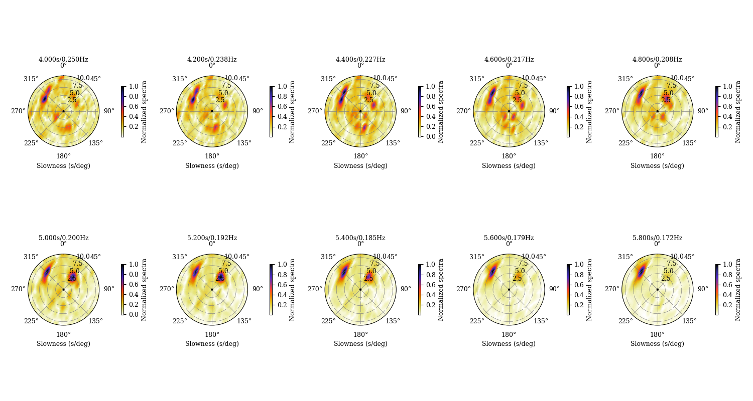
Cross spectral beamforming spectra are computed for every frequency and we find that there are mainly maximum spectrum regions: 7.5 and 5 $s/degree$, respectively.
 1
 2
 3
 4
 5
 6
 7
 8
 9
10
11
12
13
14
15
16
17
18
19
20
21
22
23
24
25
26
27
28
29
30
31
32
33
34
35
36
37
38
39
40
41
42
43
44
45
46
47
48
49
50
51
52
53
54
55
56
57
58
59
60
61
62
63
64
65
66
67
68
69
70
71
72
73
74
75
76
|
import numpy as np
import matplotlib.pyplot as plt
import matplotlib as mpl
from scipy import fft
from obspy import read
from scipy import interpolate
from geopy.distance import geodesic
from obspy.taup.taup_geo import calc_dist_azi as cda

st = read('COR*.SAC')

ccf = []
pos = []
t1 = -300; t2 = 300
v = 3.5
for tr in st:
    b = tr.stats.sac.b; dt = tr.stats.delta
    x1 = tr.stats.sac.evlo; y1 = tr.stats.sac.evla
    x2 = tr.stats.sac.stlo; y2 = tr.stats.sac.stla
    _, az, _ = cda(y1, x1, y2, x2, 6371, 0)
    az = az / 180 * np.pi
    dist = geodesic((y1, x1), (y2, x2), ellipsoid='WGS-84').km
    nn1 = int((dist/v-b)/dt)
    nn2 = int((-dist/v-b)/dt)
    tr.data[: nn2] = 0.; tr.data[nn1: ] = 0.
    n1 = int((t1-b)/dt); n2 = int((t2-b)/dt)
    d = tr.data[n1: n2+1]; n = len(d)
    fd = np.fft.fft(np.fft.fftshift(d))
    ccf.append(fd); pos.append([np.sin(az)*dist, np.cos(az)*dist])
ccf = np.array(ccf); pos = np.array(pos) * 1e3

nf = len(ccf[0])
fs = 1 / dt
s1 = 0; s2 = 1e-4
#s1 = 2e-4; s2 = 5e-4
sn = 51; bn = 121
slow = np.linspace(s1, s2, sn)
baz = np.radians(np.linspace(0, 360, bn))
#T = np.linspace(5, 50, 10)
T = np.linspace(4, 5.8, 10)
g = 111.19492664455

plt.figure(figsize=(15, 8))
for ti, tt in enumerate(T):
    ff = 1 / tt; w = 2 * np.pi * ff
    print('Scaning period:', tt, 's ...')
    fn = int(ff*nf/fs)
    P1 = np.zeros((sn, bn), dtype=complex)
    tmp = -1j * w
    for i, ss in enumerate(slow):
        for j, bb in enumerate(baz):
            shift = ss * (-np.sin(bb)*pos[:, 0] - np.cos(bb)*pos[:, 1])
            P1[i, j] = np.dot(ccf[:, fn], np.exp(tmp*shift))
    PP = abs(P1)
    bazz2 = np.linspace(baz[0], baz[-1], 241)
    sloww2 = np.linspace(slow[0], slow[-1], 201)
    inp = interpolate.interp2d(baz, slow, PP, kind='cubic')
    PP = inp(bazz2, sloww2)
    PP = PP / PP.max()
    index = np.unravel_index(PP.argmax(), PP.shape)
    ax1 = plt.subplot(2, 5, ti+1, projection='polar')
    plt.pcolormesh(bazz2, sloww2*1e3*g, PP, cmap='CMRmap_r')
    cbar = plt.colorbar(shrink=0.25, pad=0.2)
    cbar.set_label(r'Normalized spectra', fontsize=9)
    cbar.ax.tick_params(labelsize=9)
    ax1.grid(color='gray', ls=(2, (30, 5)), lw=0.5)
    ax1.tick_params(axis='y', colors='k', labelsize=9)
    ax1.set_theta_zero_location('N')
    ax1.set_theta_direction(-1)
    ax1.plot(baz, np.ones(len(baz))*slow.min()*1e3, c='k', lw=2)
    ax1.plot(baz, np.ones(len(baz))*slow.max()*1e3, c='k', lw=2)
    ax1.set_xlabel('Slowness (s/deg)', fontsize=9)
    plt.xticks(fontsize=9); plt.yticks(fontsize=9)
    plt.title('%.3fs/%.3fHz'%(tt,1/tt), fontsize=9, pad=15)
plt.tight_layout()
plt.show()
|
We think they are body waves originating from distant storms and more work is necessary to conduct for recognizing the body wave phases. If we assume that what the seismic phase is, we can use back-projection to find the regions of the distant storms and compare them with the significant wave height data (e. g., Gerstoft et al., 2006; Euler et al., 2017). For more details, see these research articles. Note that, how do we find the position with given back-azimuth and horizontal slowness (ray parameter) of some body phase can be figured out using some body wave ray toolkits, such as obspy (see Calculating ray parameters of body waves with obspy to find the specific steps ) or TauP.
Bibliography
Euler, G. G., Wiens, D. A., & Nyblade, A. A. (2014). Evidence for bathymetric control on the distribution of body wave microseism sources from temporary seismic arrays in africa. Geophysical Journal International , 197 (3), 1869-1883.
Gal, M. , Reading, A. M. , Ellingsen, S. P. , Koper, K. D. , Gibbons, S. J. , & SP Näsholm. (2015). Improved implementation of the fk and capon methods for array analysis of seismic noise. Geophysical Journal International(2), 1045-1054.
Gerstoft, P., M. C. Fehler, and K. G. Sabra (2006), When Katrina hit California, Geophys. Res. Lett., 33, L17308.
Gerstoft, P., P. M. Shearer, N. Harmon, and J. Zhang (2008), Global P, PP, and PKP wave microseisms observed from distant storms, Geophys. Res. Lett., 35, L23306.
Nakata, N. , Gualtieri, L. , & Fichtner, A. . (2019). Seismic Ambient Noise. P. 43$-$44.
