1. Basic descriptions
Matched filed processing (MFP) is a location algorithm that was first applied in ocean acoustics (Baggeroer and Kuperman, 1988).
It has been widely used to locate quakes or microseisms in seismology (e.g., Cros et al., 2011; Gal et al., 2018).
We here give a short and simple derivation of MFP as follows.
1.1 MFP power
Computing the Fourier spectrum vector,
$$
\boldsymbol{u}(\omega) = [u_1(\omega), u_2(\omega), \cdots, u_N(\omega)]^T, \tag{1}
$$
where, $N$ is the total number of receivers, $T$ means transpose operator, $u_i(\omega)$
is the Fourier spectrum of recordings by receiver $i$, and $\omega$ is angular frequency.
Calculating the covariance matrix,
$$
\boldsymbol{C}(\omega) = \boldsymbol{u}(\omega) \boldsymbol{u}^H(\omega), \tag{2}
$$
where, $H$ denotes the Hermitian transpose operator.
Generally, we only keep the phase information, and the covariance matrix is thus normalized as follows,
$$
\tilde{C}_{mn}(\omega) = \frac{C_{mn}(\omega)}{|C_{mn}(\omega)|}. \tag{3}
$$
Generating the steering vector,
$$
\boldsymbol{a}(\omega, v, \boldsymbol{r}) = [e^{-i\omega |\boldsymbol{r}-\boldsymbol{r}_1|/v}, e^{-i\omega |\boldsymbol{r}-\boldsymbol{r}_2|/v}, \cdots, e^{-i\omega |\boldsymbol{r}-\boldsymbol{r}_N|/v}]^T, \tag{4}
$$
in which, $v$ is the wave speed, $\boldsymbol{r}$ and $\boldsymbol{r}_i$ are the candidate source and the $i$th receiver positions, respectively.
Finally, the matched field processing coherence is defined by
$$
P(\omega, v, \boldsymbol{r}) = \frac{1}{N^2} \boldsymbol{a}^H(\omega, v, \boldsymbol{r}) \tilde{\boldsymbol{C}}(\omega) \boldsymbol{a}(\omega, v, \boldsymbol{r}). \tag{5}
$$
We may find the potential source position when the MFP coherence reaches the maximum.
The Earth’s heterogenieties of seismic wave propagation speed, however, may result in limitations of MFP in seismology. Some individuals thus consider using ray tracing for calculating travel time when three-dimensional seismic wave velocity model is involed in (Gal et al., 2018).
1.2 MFP array response function
Similar to F-K beamforming, we can give a signal with corresponding source position, wave speed and frequency
to check the resolution of our array geometry configuration.
Utilizing the wave speed $v$, source position $\boldsymbol{r}_0$ and frequency $\omega$ of the given signal,
we first construct the signal complex spectrum vector,
$$
\boldsymbol{u}(\omega, v, \boldsymbol{r}_0) = [e^{-i\omega|\boldsymbol{r}_0-\boldsymbol{r}_1|/v}, e^{-i\omega|\boldsymbol{r}_0-\boldsymbol{r}_2|/v}, \cdots, e^{-i\omega|\boldsymbol{r}_0-\boldsymbol{r}_N|/v}]^T. \tag{6}
$$
The signal convariance matrix is given by
$$
\boldsymbol{C}(\omega) = \boldsymbol{u}(\omega, v, \boldsymbol{r}_0) \boldsymbol{u}^H(\omega, v, \boldsymbol{r}_0). \tag{7}
$$
Calculating the phase information of the covariance matrix as follows,
$$
\tilde{C}_{mn}(\omega) = \frac{C_{mn}(\omega)}{|C_{mn}(\omega)|}. \tag{8}
$$
Gnerating steering vector,
$$
\boldsymbol{a}(\omega, v, \boldsymbol{r}) = [e^{-i\omega|\boldsymbol{r}-\boldsymbol{r}_1|/v}, e^{-i\omega|\boldsymbol{r}-\boldsymbol{r}_2|/v}, \cdots, e^{-i\omega|\boldsymbol{r}-\boldsymbol{r}_N|/v}]^T \tag{9}
$$
to yield the MFP coherence
$$
P(\omega, v, \boldsymbol{r}) = \frac{1}{N^2} \boldsymbol{a}^H(\omega, v, \boldsymbol{r}) \tilde{\boldsymbol{C}}(\omega) \boldsymbol{a}(\omega, v, \boldsymbol{r}). \tag{10}
$$
For simplicity, we add up coherences of different frequencies to obtain the final MFP coherence
$$
P_0(v, \boldsymbol{r}) = \frac{1}{K} \sum_{k}P(\omega_k, v, \boldsymbol{r}). \tag{11}
$$
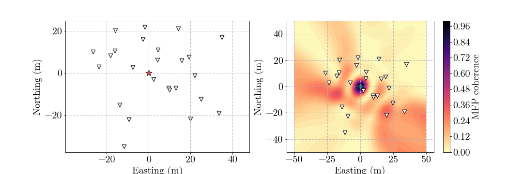
2. Numerical test: array response function
 1
 2
 3
 4
 5
 6
 7
 8
 9
10
11
12
13
14
15
16
17
18
19
20
21
22
23
24
25
26
27
28
29
30
31
32
33
34
35
36
37
38
39
40
41
42
43
44
45
46
47
48
49
50
51
52
53
54
55
56
57
58
59
60
61
62
63
64
65
66
67
68
69
|
# import required packages.
import numpy as np
import matplotlib.pyplot as plt
from geopy.distance import geodesic
from obspy import read
from mpl_toolkits.basemap import Basemap
from obspy.taup import TauPyModel
from obspy.taup.taup_geo import calc_dist

# Euclidean distances between the array and 2D-shape postions.
def cartesian_distance_matrix(X, Y, xy):
    nr = xy.shape[0]
    ny, nx = X.shape
    r = np.zeros((nr, ny, nx))
    for i in range(nr):
        r[i] = ( (X-xy[i, 0])**2 + (Y-xy[i, 1])**2 ) ** 0.5
    return r

def mfp_array_response(xy, f0=20, v0=500, x0=0, y0=0, x1=-100, x2=100, nx=51, y1=-100, y2=100, ny=51):
    nr = xy.shape[0]
    tmp = -2j * np.pi * f0 / v0
    r = ( (x0-xy[:, 0])**2 + (y0-xy[:, 1])**2 ) ** 0.5
    u = np.exp(tmp*r); u = u.reshape((nr, 1))
    c0 = u @ np.conjugate(u.T)
    c0 /= np.abs(c0); c0[np.isnan(np.abs(c0))] = 0.
    x = np.linspace(x1, x2, nx); y = np.linspace(y1, y2, ny)
    X, Y = np.meshgrid(x, y)
    p = np.zeros((ny, nx), dtype=complex)
    r = cartesian_distance_matrix(X, Y, xy)
    for i in range(nr):
        for j in range(nr):
            p += (c0[i, j] * np.exp(tmp*(r[j]-r[i])))
    return x, y, np.abs(p)/nr**2


f0 = 20; v0 = 500
x0 = 0; y0 = 0
x1 = -50; x2 = 50; nx = 51
y1 = -50; y2 = 50; ny = 51

nr = 25; r = 35
xy = np.random.randn(nr, 2)
xy[:, 0] /= np.abs(xy[:, 0]).max()
xy[:, 1] /= np.abs(xy[:, 1]).max()
xy *= r

x, y, p = mfp_array_response(xy, f0=f0, v0=v0, x0=x0, y0=y0, x1=x1, x2=x2, nx=nx,
                            y1=y1, y2=y2, ny=ny)

plt.figure(figsize=(15, 5))
plt.subplot(121)
plt.scatter(xy[:, 0], xy[:, 1], marker='v', s=75, facecolor='#EEEEEE', edgecolor='k')
plt.scatter(x0, y0, marker='*', s=200, facecolor='r', edgecolor='k', alpha=0.75)
plt.xlabel('Easting (m)')
plt.ylabel('Northing (m)')
plt.grid(ls=(8, (6, 3)))
plt.axis('equal')

plt.subplot(122)
plt.contourf(x, y, p, cmap='magma_r', levels=51)
cbar = plt.colorbar()
cbar.set_label('MFP coherence')
plt.scatter(xy[:, 0], xy[:, 1], marker='v', s=75, facecolor='#EEEEEE', edgecolor='k')
plt.plot(x0, y0, 'cx', lw=2.5)
plt.xlabel('Easting (m)')
plt.ylabel('Northing (m)')
plt.grid(ls=(8, (6, 3)))
plt.axis('equal')
plt.show()
|
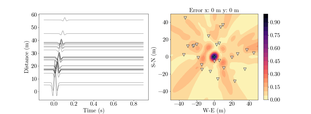
3. Numerical example: locate source using synthetic data
We synthesize waveform data utilizing time shift according to distances between receivers and the source.
 1
 2
 3
 4
 5
 6
 7
 8
 9
10
11
12
13
14
15
16
17
18
19
20
21
22
23
24
25
26
27
28
29
30
31
32
33
34
35
36
37
38
39
40
41
42
43
44
45
46
47
48
49
50
51
52
53
54
55
56
57
58
59
60
61
62
63
64
65
66
67
68
69
70
71
72
73
74
75
76
77
78
79
80
81
82
83
84
|
def cartesian_mfp_data(C, f, xy, v, x1=0, x2=500, y1=0, y2=500, nx=101, ny=101):
    nr = xy.shape[0]
    x = np.linspace(x1, x2, nx)
    y = np.linspace(y1, y2, ny)
    X, Y = np.meshgrid(x, y)
    r = cartesian_distance_matrix(X, Y, xy)
    tmp = -2j * np.pi * f / v
    p = np.zeros((ny, nx), dtype=complex)
    for i in range(nr):
        for j in range(nr):
            p += (C[i, j]*np.exp(tmp*(r[j]-r[i])))
    return x, y, np.abs(p)/nr**2

# Generate receiver and source positions.
nr = 25; r = 45
xy = np.random.randn(nr, 2)
xy[:, 0] /= np.abs(xy[:, 0]).max()
xy[:, 1] /= np.abs(xy[:, 1]).max()
xy *= r
src = np.array([0, 0])

# Synthesize waveforms and computing Fourier spectrum.
n = 501; dt = 2e-3
f0 = 20; v0 = 500
t = np.arange(n) * dt - 2/f0
# Ricker wavelet.
s = (1-2*(np.pi*f0*t)**2) * np.exp(-(np.pi*f0*t)**2)
data = np.zeros((nr, n))
r = np.zeros(nr)
fd = []
# Shifting signal accroding to distance between the receiver and source.
for i in range(nr):
    tmp = src - xy[i]
    r[i] = np.dot(tmp, tmp)**0.5
    index = int(r[i]/v0/dt)
    if index < 0:
        index = 0
    data[i, index: index+100] = s[:100] / r[i]
    fd.append(np.fft.fft(data[i]))
fd = np.array(fd)

# Parameters of processing.
nf = fd.shape[1]
f1 = 20; f2 = 30; fs = 1 / dt
fn1 = int(f1*nf/fs)
fn2 = int(f2*nf/fs)
x1 = -50; x2 = 50; nx = 51
y1 = -50; y2 = 50; ny = 51

# Processing
p0 = np.zeros((ny, nx))
for i in range(fn1, fn2+1):
    f = i * fs / nf
    u = fd[:, i]; u = u.reshape((nr, 1))
    C = u @ np.conjugate(u.T)
    C /= np.abs(C); C[np.isnan(np.abs(C))] = 0.
    x, y, p = cartesian_mfp_data(C, f, xy, v0, x1=x1, x2=x2, y1=y1, y2=y2, nx=nx, ny=ny)
    p0 += p
p0 /= (fn2-fn1+1)


# Waveforms.
scale = 100
plt.figure(figsize=(15, 4.5))
plt.subplot(121)
for i in range(nr):
    plt.plot(t, data[i]*scale+r[i], 'k', lw=0.5)
plt.xlabel('Time (s)')
plt.ylabel('Distance (m)')

# Matched field processing coherence.
plt.subplot(122)
index = np.argmax(p0)
xi = index % nx; yi = index // nx
plt.contourf(x, y, p0, cmap='magma_r', levels=21, zorder=0)
plt.colorbar()
plt.scatter(xy[:, 0], xy[:, 1], marker='v', s=100,
            facecolor='#DDDDDD', edgecolor='k', lw=1, alpha=0.75, zorder=2)
plt.scatter(src[0], src[1], marker='x', s=100, color='c', lw=1, alpha=0.9, zorder=3)
plt.title('Error x: %g m y: %g m'%(x[xi]-src[0], y[yi]-src[1]))
plt.xlabel('W-E (m)')
plt.ylabel('S-N (m)')
plt.axis('equal')
plt.show()
|
4. Locating a source using seismic wave with period of hundreds of seconds
4.1 MFP array response function of a seismic network of GSN, IU
 1
 2
 3
 4
 5
 6
 7
 8
 9
10
11
12
13
14
15
16
17
18
19
20
21
22
23
24
25
26
27
28
29
30
31
32
33
34
35
36
37
38
39
40
41
42
43
44
45
46
47
48
49
50
51
52
53
54
55
56
57
58
59
60
61
62
63
64
65
66
67
68
69
70
71
72
73
74
75
76
77
78
79
|
# Calculating distances between the seismic array and 2D-array positions.
def lonlat_distance_matrix(X, Y, xy, R=6.371e6):
        d2r = np.pi / 180
        nr = xy.shape[0]
        ny, nx = X.shape
        r = np.zeros((nr, ny, nx))
        for i in range(nr):
                dlo = (xy[i, 0] - X) * d2r
                dla = (xy[i, 1] - Y) * d2r
                a = np.sin(dla / 2) ** 2 + np.cos(Y * d2r) * np.cos(xy[i, 1] * d2r) * np.sin(dlo / 2) ** 2
                c = 2 * np.arctan2(a ** 0.5, (1 - a) ** 0.5)
                r[i] = c * R
        return r

def geographical_mfp_array_response(lola, f0=3e-3, v0=4.5e3, lo0=0, la0=0, lo1=-180, lo2=180, nlo=91, la1=-90, la2=90, nla=46):
    nr = lola.shape[0]
    r = np.zeros(nr)
    p0 = (la0, lo0)
    # Calculate distances from the source to the array.
    for i in range(nr):
        p1 = (lola[i, 1], lola[i, 0])
        r[i] = geodesic(p0, p1, ellipsoid='WGS-84').km * 1e3
    # Generate signal covariance matrix with given frequency, wave speed and position.
    tmp = -2j * np.pi * f0 / v0
    u = np.exp(tmp*r); u = u.reshape((nr, 1))
    c0 = u @ np.conjugate(u.T); c0 /= np.abs(c0); c0[np.isnan(np.abs(c0))] = 0.
    lo = np.linspace(lo1, lo2, nlo)
    la = np.linspace(la1, la2, nla)
    LO, LA = np.meshgrid(lo, la)
    r = lonlat_distance_matrix(LO, LA, lola)
    # Searching all potential source positions.
    p = np.zeros((nla, nlo), dtype=complex)
    for i in range(nr):
        for j in range(nr):
            p += c0[i, j]*np.exp(tmp*(r[j]-r[i]))
    return lo, la, np.abs(p)/nr**2


# Freqyency and wave speed of the given signal.
f0 = 2.5e-3; v0 = 5.2e3
# Source position.
lo0 = 0; la0 = 0
# Longitude and latitude ranges for searching.
lo1 = -180; lo2 = 180; nlo = 91
la1 = -90; la2 = 90; nla = 46

# Read in seismic array coordinates.
lola = []
with open('data/large_earthquakes/2010-02-27/IU.txt', 'r') as fin:
    for line in fin.readlines():
        tmp = line.strip().split('|')
        lola.append([float(tmp[3]), float(tmp[2])])
lola = np.array(lola)

# Computing matched field processing coherence.
lo, la, p = geographical_mfp_array_response(lola, f0=f0, v0=v0, lo0=lo0, la0=la0,
                                            lo1=lo1, lo2=lo2, nlo=nlo,
                                            la1=la1, la2=la2, nla=nla)


# Visualization.
plt.figure(figsize=(12, 6))
bmap = Basemap(projection='cyl', lon_0=0)
bmap.shadedrelief(scale=0.2)
X, Y = np.meshgrid(lo, la)
X, Y = bmap(X, Y)
bmap.contourf(X, Y, p, cmap='magma_r', levels=21, alpha=0.5)
cbar = plt.colorbar(shrink=0.82, pad=0.05)
cbar.ax.tick_params(labelsize=12)
cbar.set_label('MFP coherence')
xx, yy = bmap(lola[:, 0], lola[:, 1])
bmap.scatter(xx, yy, marker='v', s=100, facecolor='#EEEEEE', edgecolor='k')
xx, yy = bmap(lo0, lo0)
bmap.scatter(xx, yy, marker='x', s=200, facecolor='c', alpha=0.5)
bmap.drawparallels(circles=np.linspace(-90, 90, 7), labels=[1, 0, 0, 0], fontsize=20)
bmap.drawmeridians(meridians=np.linspace(-180, 180, 7), labels=[0, 0, 0, 1], fontsize=20)
plt.show()
|
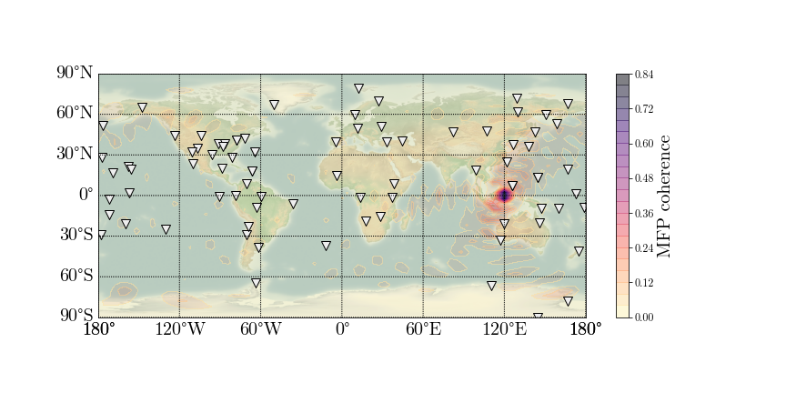
The above figure shows us that the geometry configuration of network IU has a good resolution for a given signal
that has a wave speed of 5.2 km/s and locate at (120, 0).
4.2 Searching the epicenter of Chile earthquake on Feb 27, 2010 using surface waves
 1
 2
 3
 4
 5
 6
 7
 8
 9
10
11
12
13
14
15
16
17
18
19
20
21
22
23
24
25
26
27
28
29
30
31
32
33
34
35
36
37
38
39
40
41
42
43
44
45
46
47
48
49
50
51
52
53
54
55
56
57
58
59
60
61
62
63
64
65
66
67
68
69
70
71
72
73
74
75
76
77
78
79
80
81
82
83
84
85
86
|
def geographical_mfp_data(fd, lola, f, fs, v, lo1=-180, lo2=180, nlo=91, la1=-90, la2=90, nla=46):
    nr = lola.shape[0]
    lo = np.linspace(lo1, lo2, nlo)
    la = np.linspace(la1, la2, nla)
    LO, LA = np.meshgrid(lo, la)
    p0 = np.zeros((nla, nlo))
    r = lonlat_distance_matrix(LO, LA, lola)
    for fn, ff in enumerate(f):
        tmp = -2j * np.pi * ff / v[fn]
        u = fd[:, fn]; u = u.reshape((nr, 1))
        cov = u @ np.conjugate(u.T); cov /= np.abs(cov); cov[np.isnan(np.abs(cov))] = 0.
        p = np.zeros((nla, nlo), dtype=complex)
        for i in range(nr):
            for j in range(nr):
                p += (cov[i, j]*np.exp(tmp*(r[j]-r[i])))
        p0 += np.abs(p)
    return lo, la, p0/(nr**2*len(f))


# Surface wave dispersion data.
disp = np.loadtxt('data/hum_dispersion.txt')
# Frequency range.
f1 = 2.5e-3; f2 = 3e-3
fn1 = int((f1-disp[0, 0])/(disp[1, 0]-disp[0, 0]))
fn2 = int((f2-disp[0, 0])/(disp[1, 0]-disp[0, 0]))
sta = {}
# Longitudes and latitudes of seismic stations in IU.
with open('data/large_earthquakes/2010-02-27/IU.txt', 'r') as fin:
    for line in fin.readlines():
        tmp = line.strip().split('|')
        sta[tmp[0]+'.'+tmp[1]] = [float(tmp[3]), float(tmp[2])]

lola = []
fd = []
t1 = 0; t2 = 10000
# Read in seismic data.
st = read('data/large_earthquakes/2010-02-27/IU.*.SAC')
for tr in st:
    k = tr.stats.network + '.' + tr.stats.station
    x, y = sta[k]
    n1 = int((t1-tr.stats.sac.b)/tr.stats.delta)
    n2 = int((t2-tr.stats.sac.b)/tr.stats.delta)
    d = tr.data[n1: n2+1] - tr.data[n1: n2+1].mean()
    fd.append(np.fft.fft(d))
    lola.append([x, y])
lola = np.array(lola)
fd = np.array(fd)
nf = fd.shape[1]
fs = 1 / tr.stats.delta
f = np.arange(nf) * fs / nf
fn1 = int(f1*nf/fs)
fn2 = int(f2*nf/fs)
# Obtain phase velocity.
v = []
for fn in range(fn1, fn2+1):
    n0 = int((f[fn]-disp[0, 0])/(disp[1, 0]-disp[0, 0]))
    v.append(disp[n0, 1])
v = np.array(v) * 1e3
# Searching parameters.
lo1 = -180; lo2 = 180; nlo = 181
la1 = -90; la2 = 90; nla = 91
# Computing matched field processing coherences.
lo, la, p = geographical_mfp_data(fd[:, fn1: fn2+1], lola,f[fn1: fn2+1], fs, v,
                                  lo1=lo1, lo2=lo2, nlo=nlo, la1=la1, la2=la2, nla=nla)


# Real epicenter of this earthquake.
la0, lo0 = -36.1485, -72.9327

plt.figure(figsize=(12, 6))
bmap = Basemap(projection='cyl', lon_0=0)
bmap.shadedrelief(scale=0.2)
X, Y = np.meshgrid(lo, la)
X, Y = bmap(X, Y)
bmap.contourf(X, Y, p, cmap='magma_r', levels=21, alpha=0.45)
cbar = plt.colorbar(shrink=0.82, pad=0.05)
cbar.ax.tick_params(labelsize=12)
cbar.set_label('MFP coherence')
xx, yy = bmap(lola[:, 0], lola[:, 1])
bmap.scatter(xx, yy, marker='v', s=50, facecolor='#EEEEEE', edgecolor='k')
xx, yy = bmap(lo0, la0)
bmap.scatter(xx, yy, marker='x', s=150, facecolor='c', lw=2)
bmap.drawparallels(circles=np.linspace(-90, 90, 7), labels=[1, 0, 0, 0], fontsize=20, color='none')
bmap.drawmeridians(meridians=np.linspace(-180, 180, 7), labels=[0, 0, 0, 1], fontsize=20, color='none')
plt.savefig(r'F:\Hugo_Web\Hugo_Blogs_Geophydog\static\Array_Processing\MFP_IU_Chile.png')
plt.show()
|
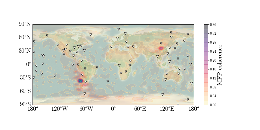
The result gives the coherence maximum position near the real epicenter. There is, however,
a obvious local coherence minimum at the antipodal position in China, which is reasonable
on account of global propogation of surface waves with period of hundreds of seconds.
5. Icequake localizations of a glacier in the French Alps
Icequakes frequently happen in s glacial system when englacial fracture propagation (e.g., Walter et al., 2009)
or basal processes (Winbery et al., 2013) exist. Here we utilize MFP algorithm to localize some icequakes in
Glacier d’Argentière (France). A dense seismic array was installed to sample quake signals or ambient noise.
The icequake localization is a 4-parameter (two position components, elevation and speed of wave propagation)
problem although we simplify the velocity of wave propagation as an one-demensional model.
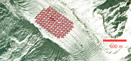
We here consider a two-parameter grid-searching model to find the potential source position (x, y).
The surface wave propagation speed is about 1600 m/s in ice from phase velocity measurements based on
ambient noise interferometry (Sergeant ey al., 2020), and we assume that the source is near surface.
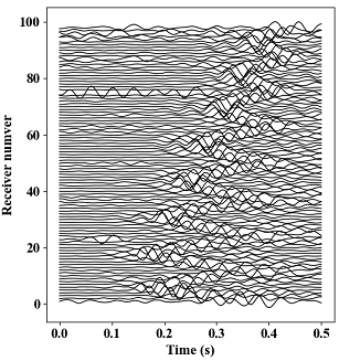
We collected seismic data between 2018-05-06T18:35:51.000 and 2018-05-06T18:35:51.5 to perform this
source position searching, and the main frequency band of this icequake event is from 10 to 30 Hz.
 1
 2
 3
 4
 5
 6
 7
 8
 9
10
11
12
13
14
15
16
17
18
19
20
21
22
23
24
25
26
27
28
29
30
31
32
33
34
35
36
37
38
39
40
41
42
43
44
45
46
47
48
49
50
51
52
53
54
55
56
57
58
59
60
61
62
63
64
65
66
67
68
69
70
71
72
73
74
75
76
77
78
79
80
81
82
83
84
85
|
from obspy import read
import numpy as np
import matplotlib.pyplot as plt
from glob import glob

def mfp_2d(C, f, xy, v, e, x1=0, x2=500, y1=0, y2=500, nx=101, ny=101):
    n = len(xy[:, 0])
    p = np.zeros((ny, nx), dtype=complex)
    x = np.linspace(x1, x2, nx)
    y = np.linspace(y1, y2, ny)
    tmp = -2j * np.pi * f / v
    for i in range(ny):
        yy = y[i]
        for j in range(nx):
            xx = x[j]
            r = np.array([((xx-xy[l][0])**2+(yy-xy[l][1])**2+(e-xy[l][2])**2)**0.5 for l in range(n)])
            a = np.exp(tmp*r)
            a = a.reshape((n, 1))
            p[i, j] = np.conjugate(a.T) @ C @ a

    return x, y, p


def main():
    t1 = 2151; t2 = 2151.5
    files = sorted(glob('data/hour-18*.AR0*.SAC'))
    sta = {}
    with open('sta.lst', 'r') as fin:
        for line in fin.readlines():
            tmp = line.strip().split()
            sta[tmp[0]] = [float(dd) for dd in tmp[1: 4]]
    fd = []; xy = []
    for fi, ff in enumerate(files):
        tr = read(ff)[0]
        dt = tr.stats.delta
        b = tr.stats.sac.b
        n1 = int((t1-b)/dt); n2 = int((t2-b)/dt)
        d = tr.data[n1: n2+1]
        d -= d.mean(); d /= np.abs(d).max()
        fd.append(np.fft.fft(d))
        k = tr.stats.station
        xy.append(sta[k])
    fd = np.array(fd)
    xy = np.array(xy)
    nf = len(fd[0])
    fs = 1 / tr.stats.delta
    v = 1640; e = 2370
    f1 = 10; f2 = 30
    fn1 = int(f1*nf/fs);
    fn2 = int(f2*nf/fs);
    tmp = ff.split('/')[0].split('_')

    levels = 51
    x1 = -750; x2 = 750;  nx = 151
    y1 = -500; y2 = 500;  ny = 101
    n = xy.shape[0]
    for i in range(fn1, fn2+1):
        f = i * fs / nf
        print('Processing at frequency %.2f Hz ...'%f)
        u = fd[:, i]; u = u.reshape((n, 1))
        C = u @ np.conjugate(u.T); C /= np.abs(C)
        x, y, p = mfp_2d(C, f, xy, v, e, x1=x1, x2=x2, y1=y1, y2=y2, nx=nx, ny=ny)
        p = np.abs(p)
        if i == fn1:
            p0 = np.zeros_like(p)
        p0 += p

    P = p0 / (fn2-fn1+1) / n ** 2
    index = np.argmax(P)
    xi = index % nx; yi = index // nx
    plt.figure(figsize=(10, 5.5))
    plt.contourf(x, y, P, cmap='magma_r', levels=levels, zorder=0)
    cbar = plt.colorbar()
    cbar.ax.tick_params(labelsize=9)
    plt.scatter(xy[:, 0], xy[:, 1], marker='o', s=50, color='k', alpha=0.25, zorder=2)
    plt.scatter(x[xi], y[yi], marker='x', s=10, color='w', alpha=0.5, zorder=3)
    plt.xlabel('W-E (m)', fontsize=15)
    plt.ylabel('S-N (m)', fontsize=15)
    plt.xticks(fontsize=13)
    plt.yticks(fontsize=13)
    plt.text(x1+20, y2-80, '%.2f-%.2f Hz: %.0f %.0f'%(f1, f2, x[xi], y[yi]), fontdict={'size': 12})
    plt.show()
    print('%d %d'%(x[xi], y[yi]))

main()
|
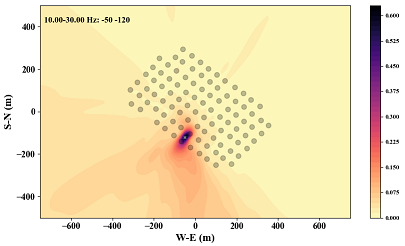
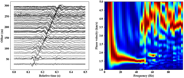
The result shows that the MFP coherence reaches maximum at (-50, -120), and we show the waveforms plotted with
increasing distances according to the source position.
Finally, we compute the frequency-phase velocity dispersion diagram using the frequency-Bessel transform (Wang et al., 2019).
Bibliography
Baggeroer, A. B., Kuperman, W. A., & Schmidt, H. (1988). Matched field processing: Source localization in correlated noise as an optimum parameter estimation problem. The Journal of the Acoustical Society of America, 83(2), 571-587.
Cros, E., Roux, P., Vandemeulebrouck, J., & Kedar, S. (2011). Locating hydrothermal acoustic sources at Old Faithful Geyser using matched field processing. Geophysical Journal International, 187(1), 385-393.
Gal, M., Reading, A. M., Rawlinson, N., & Schulte‐Pelkum, V. (2018). Matched field processing of three‐component seismic array data applied to Rayleigh and Love microseisms. Journal of Geophysical Research: Solid Earth, 123(8), 6871-6889.
Sergeant, A., Chmiel, M., Lindner, F., Walter, F., Roux, P., Chaput, J., … & Mordret, A. (2020). On the Green’s function emergence from interferometry of seismic wave fields generated in high-melt glaciers: implications for passive imaging and monitoring. The Cryosphere, 14(3), 1139-1171.
Walter, F., Clinton, J., Deichmann, N., Dreger, D. S., Minson, S., and Funk, M.: Moment tensor inversions of icequakes on
Gornergletscher, Switzerland, B. Seismol. Soc. Am., 99, 852–870, 2009.
Wang, J., Wu, G., & Chen, X. (2019). Frequency‐Bessel transform method for effective imaging of higher‐mode Rayleigh dispersion curves from ambient seismic noise data. Journal of Geophysical Research: Solid Earth, 124(4), 3708-3723.
Winberry, P., Anandakrishnan, S., Wiens, D., and Alley, R.: Nucleation and seismic tremor associated with the glacial earthquakes
of Whillans Ice Stream, Antarctica, Geophys. Res. Lett., 40, 312–315, 2013.
