1. MUSIC algorithm

The naive beamforming technique, Bartlett beamformer, has a poor resolution although its stability and robustness are good. Schmidt proposed a new beamformer algorithm call multiple signal classification (MUSIC) for addressing the resolution while keeping the stability of beamformer (1986). Here we briefly introduce the MUSIC algorithm and also give some Python codes to show how this technique works.

Assuming a signal $u(t)$ and its Fourier spectrum $U(\omega)$ of a receiver, we have a signal vector of an array composed of $N$ receivers at frequency $\omega$. $$ \vec{u}(\omega) = [U_1(\omega), U_2(\omega), \cdots, U_N(\omega)]^T \tag{1}. $$ Generally, the correlation matrix is given by $$ \bar{C}(\omega) = \frac{1}{N}\vec{u}(\omega) \vec{u}^H(\omega) \tag{2}, $$ in which $H$ denotes the Hermitian transpose operator. The correlation matrix $\bar{C}(\omega)$ is contaminated by noise arising from non-coherent signals or even instruments. The coherence signal is sotred in the correlation matrix. Thus, this matrix includes coherent signal subspace and noise subspace. Let us perform eiegendecomposition of $\bar{C}(\omega)$, resulting in the following decompositio:

$$ \bar{C}(\omega) = \bar{E}(\omega) \bar{\Lambda}(\omega) \bar{E}^{-1}(\omega) \tag{3} $$

with $\bar{E}(\omega)$ composed by $N$ eigenvectors $\vec{e}_i$ of $\bar{C}(\omega)$

$$ \bar{E}(\omega) = [\vec{e}_1, \vec{e}_2, \cdots, \vec{e}_N] \tag{4}. $$

and $\bar{\Lambda}(\omega)$ the diagonal matrix whose diagonal elements are these eigenvalues $\lambda_i$ of $\bar{C}(\omega)$

$$ \bar{\Lambda}(\omega) = diag \{ \lambda_1, \lambda_2, \cdots, \lambda_N \} \tag{5}. $$

The largest eigenvalue and its corresponding indicate the coherent signal (there may be more than one coherent signal), and the left eigenvalues and their eigenvectors are occupied by noise, which means these noise are orthogonal. Here we construct a new matrix using eigenvectors of noise,

$$ \bar{N}_e(\omega) = [\vec{e}_1, \vec{e}_2, \cdots, \vec{e}_{ne}] [\vec{e}_1, \vec{e}_2, \cdots, \vec{e}_{ne}]^H \tag{6}. $$

We change the form of Barlett beamformer

$$ P(\omega) = \vec{a}(\omega) \bar{C}(\omega) \vec{a}^H(\omega) \tag{7} $$

into

$$ P(\omega) =\frac{1}{ \vec{a}(\omega) \bar{N}_e(\omega) \vec{a}^H(\omega) } \tag{8}, $$ with $\vec{a}(\omega)$ denoteing the steering vector $\vec{a}_n=e^{-i\omega \Delta t_n}$. The denominator term of formula $(8)$ will be zero when we project the steering vector onto the noise matrix subspace spanned by eigenvectors of noise. In such cases, $P(\omega)$ will take a very large value, which is a peak case in the function $P(\omega)$.

$\Delta t_n$ is the time delay with a form of

$$ \Delta t_n = \vec{s} \cdot \vec{r}_n \tag{9} $$

for the beamforming array processing and

$$ \Delta t_n = \frac{|\vec{r}_s-\vec{r}_n|}{v} \tag{10} $$ for the matched field processing source location technique.

$\vec{s}=s[-sin\theta, -cos\theta]^T$ and $\vec{r}_n$ are separately the slowness vector of signal incoming from the back-azimuth $\theta$ and position vector of receiver $n$ in formula $(9)$.

$\vec{r}_s$ and $v$ in formula $(10)$ are the source position vector and the propagation speed of signal, respectively.

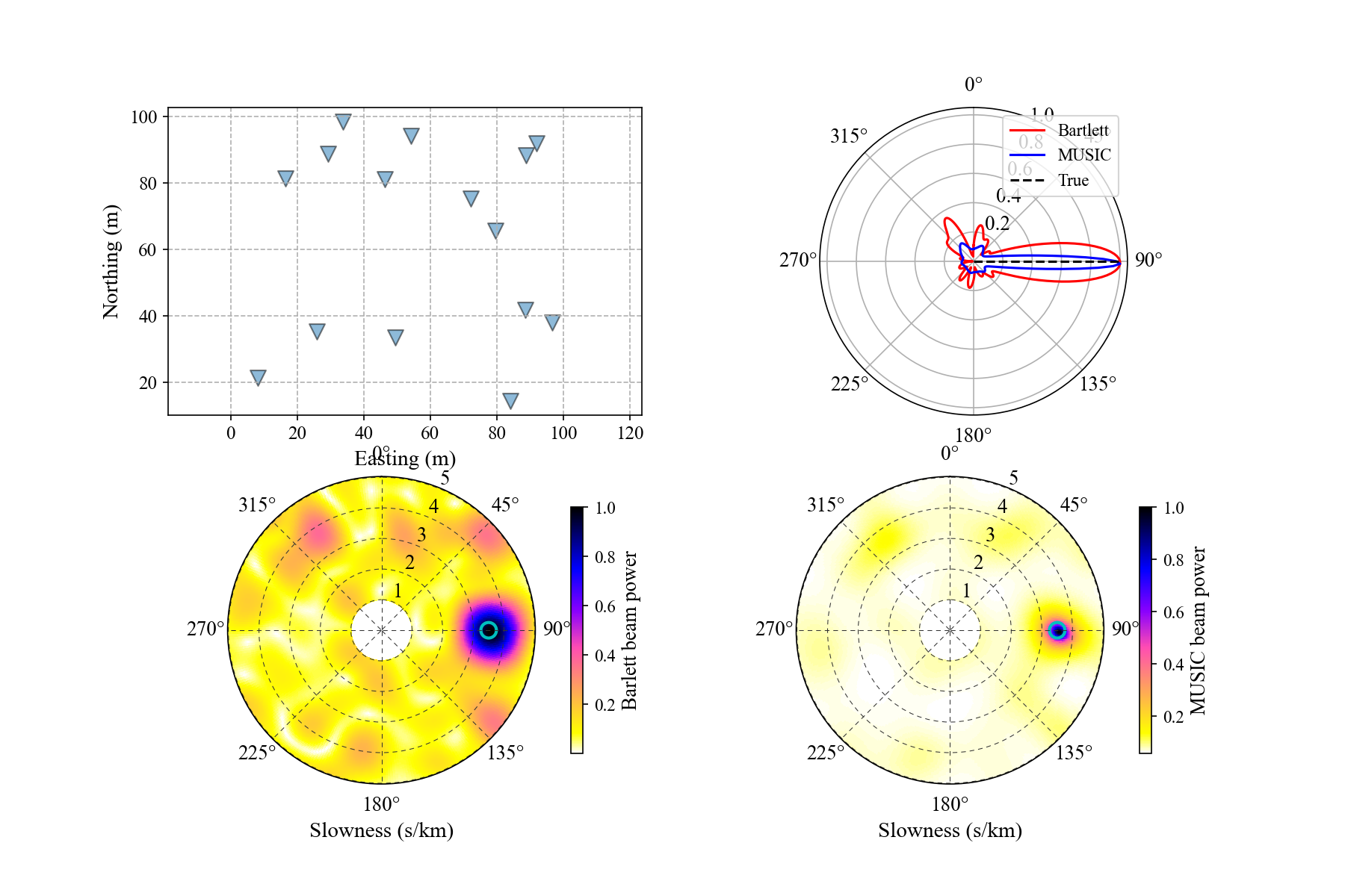
The MUSIC algorithm is better than the Bartlett beamformer in resolution. The Bartlett beamformer, however, has a better robustness compared with MUSIC. We will show some examples to validate these two algorithms using the following Python codes.

2. Array Response Functions (ARF) of Bartlett and MUSIC Beamformer.

We randomly generate an array of Cartician coordinates with $N$ elements. First we implement the array response functions of the Bartlett and the MUSIC beamformers to check their resolution and robustness.

 1
 2
 3
 4
 5
 6
 7
 8
 9
10
11
12
13
14
15
16
17
18
19
20
21
22
23
24
25
26
27
28
29
30
31
32
33
34
35
36
import numpy as np
import matplotlib.pyplot as plt

# ARF of the Bartlett beamformer.
def arf_beam_barlett(c0, xy, f0=10, b0=90, s0=3.5e-3, b1=0, b2=360, nb=181, s1=1e-3, s2=5e-3, ns=81):
    n = xy.shape[0]
    a = np.zeros((n, 1), dtype=complex)
    b = np.linspace(b1, b2, nb)
    bb = np.radians(b)
    s = np.linspace(s1, s2, ns)
    p = np.zeros((ns, nb), dtype=complex)
    for i in range(ns):
        for j in range(nb):
            shift = -s[i] * (np.sin(bb[j])*xy[:, 0]+np.cos(bb[j])*xy[:, 1])
            a[:, 0] = np.exp(-2j*np.pi*f0*shift)
            p[i, j] = np.conjugate(a.T) @ c0 @ a
    return b, s, p/n**2

# ARF of the MUSIC beamformer.
def arf_beam_music(c0, xy, f0=10, b0=90, s0=3.5e-3, b1=0, b2=360, nb=181, s1=1e-3, s2=5e-3, ns=81, ne=10):
    n = xy.shape[0]
    a = np.zeros((n, 1), dtype=complex)
    b = np.linspace(b1, b2, nb)
    bb = np.radians(b)
    s = np.linspace(s1, s2, ns)
    p = np.zeros((ns, nb), dtype=complex)
    w, v = np.linalg.eigh(c0)
    ve = v[:, :ne]
    ne = ve @ np.conjugate(ve.T)

    for i in range(ns):
        for j in range(nb):
            shift = -s[i] * (np.sin(bb[j])*xy[:, 0]+np.cos(bb[j])*xy[:, 1])
            a[:, 0] = np.exp(-2j*np.pi*f0*shift)
            p[i, j] = 1 / (np.conjugate(a.T) @ ne @ a)
    return b, s, p / np.abs(p).max()

Now we compute the ARF of the Barlett and MUSIC to check their resolution and accuracy.

 1
 2
 3
 4
 5
 6
 7
 8
 9
10
11
12
13
14
15
16
17
18
19
20
21
22
23
24
25
26
27
28
29
30
31
32
33
34
35
36
37
38
39
40
41
42
43
44
45
46
47
48
49
50
51
52
53
54
55
56
57
58
59
60
61
62
63
64
65
66
67
68
69
70
71
72
73
74
75
76
77
78
79
80
81
82
83
84
85
86
# Number of receivers
nr = 15
# Aperture of the array
r = 1e2
# Randomly generating the Cartician coordinates
xy = np.random.random((nr, 2)) * r
# Frequency, back-azimuth and slowness of signal
f0 = 5; b0 = 90; s0 = 3.5e-3
# From degree to radian
bb0 = np.radians(b0)
# Fourier vector if signal
u = np.zeros((nr, 1), dtype=complex)
u[:, 0] = np.exp(-2j*np.pi*f0*s0*(-np.sin(bb0)*xy[:, 0]-np.cos(bb0)*xy[:, 1]))
# Generating correlation matrix using u
c0 = u @ np.conjugate(u.T)
c0 /= np.abs(c0); c0[np.isnan(c0)] = 0.
# Back-azimuth and slowness ranges of computing
b1 = 0; b2 = 360; nb = 361
s1 = 1e-3; s2 = 5e-3; ns = 81
# Adding noise to the correlation matrix
noiser = np.random.randn(nr, nr)
noisei = np.random.randn(nr, nr)
ratio = 1.25
c0 = c0 + noiser * ratio + 1j * noisei * ratio
# Computing the Bartlett beamformer
b, s, p1 = arf_beam_barlett(c0, xy, f0=f0, b0=b0, s0=s0, b1=b1, b2=b2, nb=nb, s1=s1, s2=s2, ns=ns)
# Computing the MUSIC beamformer.
_, _, p2 = arf_beam_music(c0, xy, f0=f0, b0=b0, s0=s0, b1=b1, b2=b2, nb=nb, s1=s1, s2=s2, ns=ns, ne=nr-1)
# Normalizing beam power
p1 = np.abs(p1); p1 /= p1.max()
p2 = np.abs(p2); p2 /= p2.max()


## Visualizing the beam power results.
# Array configuration
plt.figure(figsize=(12, 8))
plt.subplot(221)
plt.scatter(xy[:, 0], xy[:, 1], marker='v', s=100, edgecolor='k', alpha=0.5)
plt.xlabel('Easting (m)', fontsize=14)
plt.ylabel('Northing (m)', fontsize=14)
plt.gca().tick_params(labelsize=12)
plt.axis('equal')
plt.grid(ls='--')

# Comparing the accuracy
sn = int((s0-s.min())/(s[1]-s[0])); dsn = 2
pp1 = np.mean(p1[sn-dsn:sn+dsn], axis=0)
pp2 = np.mean(p2[sn-dsn:sn+dsn], axis=0)
pp1 /= pp1.max(); pp2 /= pp2.max()
ax = plt.subplot(222, projection='polar')
ax.plot(np.radians(b), pp1, 'r', label='Bartlett')
ax.plot(np.radians(b), pp2, 'b', label='MUSIC')
ax.plot([np.radians(b0), np.radians(b0)], [0, 1], 'k--', label='True')
ax.legend(fontsize=11)
ax.set_theta_zero_location('N')
ax.set_theta_direction(-1)
plt.gca().tick_params(labelsize=13)

# Barlett beam power
ax = plt.subplot(223, projection='polar')
plt.pcolormesh(np.radians(b), s*1e3, p1, cmap='gnuplot2_r')
cbar = plt.colorbar(shrink=0.8, pad=0.075)
cbar.set_label(r'Barlett beam power', fontsize=13)
cbar.ax.tick_params(labelsize=11)
ax.grid(color='#333333', ls=(10, (6, 5)), lw=0.5)
ax.tick_params(axis='y', colors='k', labelsize=13)
ax.set_theta_zero_location('N')
ax.set_theta_direction(-1)
ax.set_xlabel('Slowness (s/km)', fontsize=14)
ax.tick_params(labelsize=13)
ax.scatter(bb0, s0*1e3, marker='o', s=100, facecolor='none', edgecolor='c', lw=2)

# MUSIC beam power
ax = plt.subplot(224, projection='polar')
plt.pcolormesh(np.radians(b), s*1e3, p2, cmap='gnuplot2_r')
cbar = plt.colorbar(shrink=0.8, pad=0.075)
cbar.set_label(r'MUSIC beam power', fontsize=13)
cbar.ax.tick_params(labelsize=11)
ax.grid(color='#333333', ls=(10, (6, 5)), lw=0.5)
ax.tick_params(axis='y', colors='k', labelsize=13)
ax.set_theta_zero_location('N')
ax.set_theta_direction(-1)
ax.set_xlabel('Slowness (s/km)', fontsize=14)
ax.tick_params(labelsize=13)
ax.scatter(bb0, s0*1e3, marker='o', s=100, facecolor='none', edgecolor='c', lw=2)
plt.show()

ARF_Barlett_MUSIC

References

Schmidt, R.O, “Multiple Emitter Location and Signal Parameter Estimation,” IEEE Trans. Antennas Propagation, Vol. AP-34 (March 1986), pp. 276–280.