1 Basic principles

Detection of coherent seismic signals is an interesting topic in seismology. However, it’s difficult to identify these coherent signals with single station because of the low signal to noise ratios (SNRs). Based on the array processing techniques in radial astronomy, radar and acoustics, the seismic array methods have been developed well in the past several decades. Here, we just follow the articles contributed by (Capon, 1970; Euler et al., 2014; Rost & Thomas, 2002)

$$ P(f, \vec{s}) = \sum_{i=1}^{N-1}\sum_{j=i+1}^N\omega_i \omega_j C_{ij}(f) e^{-2\pi f \vec{s} \cdot (\vec{r}_j-\vec{r}_i)} \tag{1}, $$ where, $\vec{s}$ is the slowness vector, $\omega_i$ and $\omega_j$ are the weight factors of the $i_{th}$ and $j_{th}$ stations at positions $\vec{r}_i$ and $\vec{r}_j$, respectively. $C_{ij}(f)$ is the off-diagonal element of cross spectral matrix computed with the records of stations $i,j$ at frequency $f$. $N$ is the total number of stations.

For given frequency band $[f_1, f_2]$, the sums of power over this band is given by $$ P_{all}(\vec{s}) = \sum_{f=f_1}^{f_2}P(f, \vec{s}) \tag{2}. $$

We recast slowness vector $\vec{s}$ as $$ \begin{aligned} \vec{s} &= [S_x, S_y]^T\\
&=S[cos(\alpha), sin(\alpha)]^T \\
&= S[cos(3/2\pi-\theta), sin(3/2\pi-\theta)]^T \\
&= S[-sin(\theta), -cos(\theta)]^T \end{aligned} \tag{3}, $$ where, $S=|\vec{s}|$, $\theta$ is the back-azimuth of signal source relative to the array center and $\alpha$ is the polar angle of the slowness vector. One should note that $\theta + \alpha = 3/2\pi$.

2 Numerical example

The method of implementing cross-spectral beam-forming.

 1
 2
 3
 4
 5
 6
 7
 8
 9
10
11
12
def cross_spec_bf(ccfd, pos, f, fs, s1=1e-4, s2=5e-4, b1=0, b2=360):
    w = 2 * np.pi * f; tmp = -1j * w
    nf = len(ccfd[0]); fn = int(f*nf/fs)
    nb = 121; ns = 51
    baz = np.linspace(b1, b2, nb) * np.pi / 180
    slow = np.linspace(s1, s2, ns)
    p = np.zeros((ns, nb), dtype=complex)
    for si, ss in enumerate(slow):
        for bj, bb in enumerate(baz):
            shift = ss * (-np.sin(bb)*pos[:, 0] - np.cos(bb)*pos[:, 1]) 
            p[si, bj] = sum(ccfd[:, fn]*np.exp(shift*tmp))
    return baz, slow, p

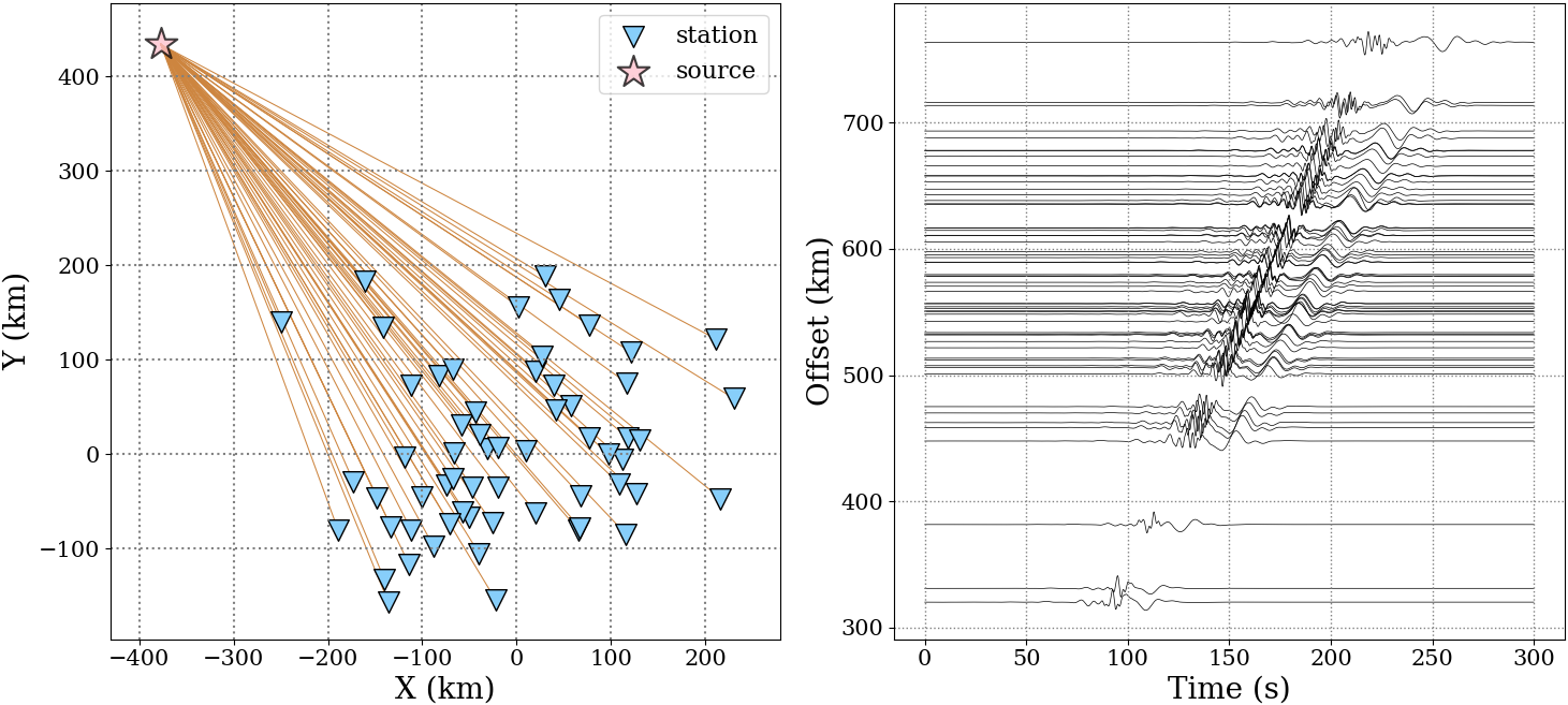
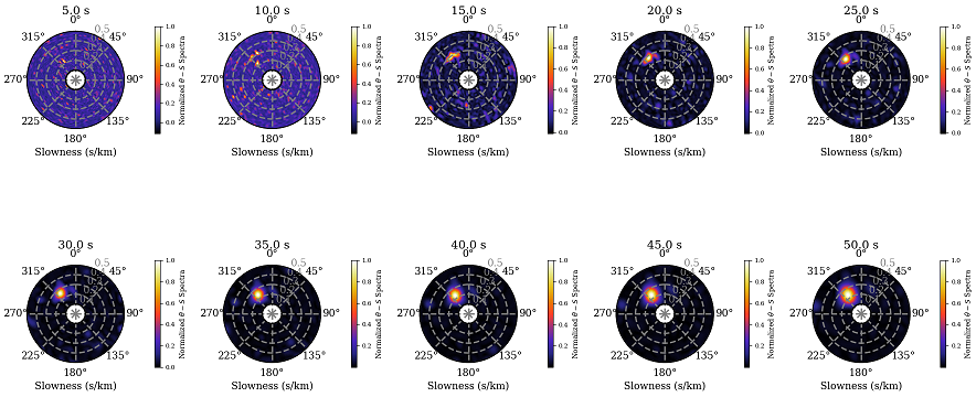
Here, we synthesize seismic traces using the CPS package (Herrmann, 2013) based on a multi-layered model. The beam-forming spectra will be computed from the synthetic seismic data.

Traces

 1
 2
 3
 4
 5
 6
 7
 8
 9
10
11
12
13
14
15
16
17
18
19
20
21
22
23
24
25
26
27
28
29
30
31
32
33
34
35
36
37
38
39
40
41
42
43
44
45
46
47
48
49
50
51
52
53
54
55
56
57
58
59
60
61
62
63
64
import numpy as np
import matplotlib.pyplot as plt
from scipy import interpolate
from obspy import read

def main():
    # Seismic data can be downloaded from "https://github.com/geophydog/Seismic_Data_Examples/Syn_Single_Seismic_Event"
    st = read('DATA/*.SAC')
    fd = []; coord = []
    for i, tr in enumerate(st):
        tr.data -= np.mean(tr.data)
        tr.detrend(); tr.data /= abs(tr.data).max()
        k = tr.stats.station
        x = tr.stats.sac.stlo
        y = tr.stats.sac.stla
        coord.append([x, y])
        tmp = np.fft.fft(tr.data)
        fd.append(list(tmp))
    fd = np.array(fd); coord = np.array(coord)
    n = len(fd[:, 0]); pos = []; ccfd = []
    for i in range(n-1):
        x1 = coord[i, 0]; y1 = coord[i, 1]
        for j in range(i+1, n):
            x2 = coord[j, 0]; y2 = coord[j, 1]
            pos.append([x2-x1, y2-y1])
            ccfd.append(fd[i]*np.conjugate(fd[j]))
    pos = np.array(pos) * 1e3
    ccfd = np.array(ccfd)
    s1 = 1e-4; s2 = 5e-4
    b1 = 0; b2 = 360
    T = np.linspace(5, 50, 10); fs = 1/ tr.stats.delta
   
    plt.figure(figsize=(18, 9.5))
    for ti, TT in enumerate(T):
        print('Scaning period %.1f s ...'%TT)
        f = 1 / TT
        baz, slow, p = cross_spec_bf(ccfd, pos, f, fs,
                                     s1=s1, s2=s2, b1=b1, b2=b2)
        PP = abs(p)
        bazz  = np.linspace(baz[0],  baz[-1], 361)
        sloww = np.linspace(slow[0], slow[-1], 201)
        inp = interpolate.interp2d(baz, slow, PP, kind='cubic')
        PP = inp(bazz, sloww)
        PP = PP / PP.max()
        ax1 = plt.subplot(2, 5, ti+1, projection='polar')
        plt.pcolormesh(bazz, sloww*1e3, PP, cmap='CMRmap')
        cbar = plt.colorbar(shrink=0.4, pad=0.2)
        cbar.set_label(r'Normalized $\theta-S$ Spectra', fontsize=9)
        cbar.ax.tick_params(labelsize=8)
        ax1.grid(color='gray', ls='--', lw=2)
        ax1.tick_params(axis='y', colors='gray', labelsize=12)
        ax1.set_theta_zero_location('N')
        ax1.set_theta_direction(-1)
        ax1.plot(baz, np.ones(len(baz))*slow.min()*1e3, c='k', lw=2)
        ax1.plot(baz, np.ones(len(baz))*slow.max()*1e3, c='k', lw=2)
        ax1.set_xlabel('Slowness (s/km)', fontsize=13)
        plt.xticks(fontsize=13); plt.yticks(fontsize=13)
        plt.title('%.1f s'%TT, fontsize=15, pad=15)
    plt.tight_layout() 
    #plt.savefig('Cross_Spectral_Beamforming.png')
    plt.show()

if __name__ == '__main__':
    main()

Beam-forming

3 The C code version

We also develop a C language version cross-spectral beam-forming, and one can find it at https://github.com/geophydog/Cross_Spectral_Beamforming.

References

Capon, J. (1970). Applications of detection and estimation theory to large array seismology. Proceedings of the IEEE, 58 (5), 760-770.

Euler, G. G., Wiens, D. A., & Nyblade, A. A. (2014). Evidence for bathymetric control on the distribution of body wave microseism sources from temporary seismic arrays in africa. Geophysical Journal International , 197 (3), 1869-1883.

Herrmann, R. B. (2013). Computer programs in seismology: An evolving tool for instruction and research. Seismological Research Letters, 84(6), 1081–1088.

Rost, S., & Thomas, C. (2002). Array seismology: Methods and applications. Reviews of geophysics, 40 (3), 2-1.