New responses between station pairs can be extracted from diffuse wave field by cross-correlating ambient seismic noise or coda (Campillo & Paul, 2003; Bensen et al., 2007). However, some processing techniques should be taken into consideration to retrieve clear emperical green’s functions (EGFs). Here we show these steps in detail.

$\boxed{\text{Data processing steps}}$

1. Cut data

2. Removing mean, trend and tapering

3. Removing instrument response

4. Band-pass filtering

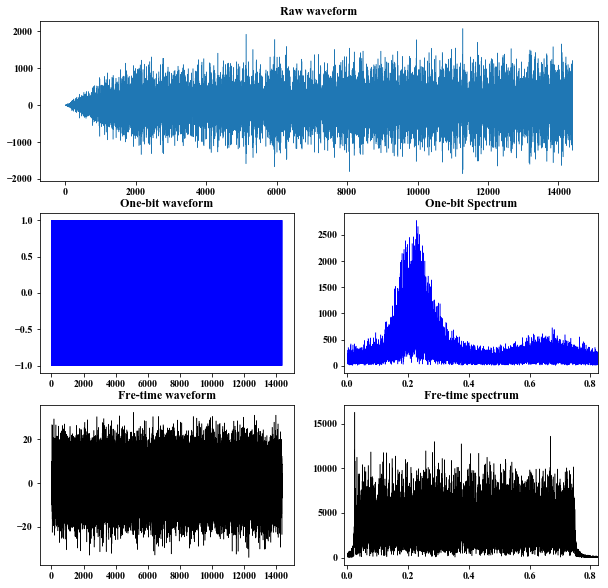
5. Temperal normalization

$\boxed{\text{One-bit}}$ $$ \tilde{d_j}=sign(d_j) \tag{1} $$ $\boxed{\text{run absolute mean}}$ $$ \begin{aligned} w_j &= \frac{1}{2N+1}\sum_{n=j-N}^{j+N}|d_n| \\
\tilde{d_j} &= \frac{d_j}{w_j} \end{aligned} \tag{2}. $$

6. Spectral whitening

Using $\text{run absolute mean}$ algorithm. $$ \begin{aligned} w_j &= \frac{1}{2N+1}|fd_j| \\
\tilde{fd_j} &= \frac{fd_j}{w_j} \end{aligned} \tag{3}. $$

Combining steps $5$ and $6$, an improved algrithm suggested by Shen et al. (2012) is given by $$ y(t) = \sum_{f_k=f_1}^{f_2}\frac{x_{f_k, f_k+\Delta f}(t)}{Env[x_{f_k,f_k+\Delta f}(t)]} \tag{4}, $$ where, in general, $\Delta f = \frac{f_1}{4}$ and $Env[x_{f_k, f_k+\Delta f}]$ is the envelope of $x_{f_k, f_k+\Delta f}(t)$.

 1
 2
 3
 4
 5
 6
 7
 8
 9
10
11
12
13
14
15
16
17
18
19
20
21
22
23
24
25
26
27
28
29
30
31
32
33
34
35
36
37
38
39
40
41
42
43
44
45
46
47
48
49
50
51
52
53
54
55
56
57
58
59
60
61
62
63
64
65
66
67
68
69
70
71
72
73
74
75
import numpy as np
from scipy.signal import butter, filtfilt
from obspy import read
import matplotlib.pyplot as plt
from scipy import fft

def envelope(d):
    fd = fft.fft(d)
    n = len(fd)
    fd[1:n//2] *= 2.
    fd[n//2:] = 0.
    return (d**2+fft.ifft(fd).imag**2)**.5

def FTN1(tr, f1, f2, num=4):
    d = np.zeros_like(tr.data)
    df = f1 / num
    fl = f1
    fh = fl + df
    while fh <= f2+df:
        trc = tr.copy()
        trc.filter('bandpass', freqmin=fl, freqmax=fh,
                   corners=4, zerophase=True)
        d += (trc.data / envelope(trc.data))
        fl += df; fh += df
    return d/(f2-f1)*df

def FTN2(d1, fs, f1, f2, num=4.):
    d2 = np.zeros_like(d1)
    df = f1 / num; fl = f1
    while fl <= f2:
        fh = fl + df
        [b, a] = butter(N=4, Wn=[2*fl/fs, 2*fh/fs], btype='bandpass')
        dd = filtfilt(b, a, d1)
        d2 += (dd/envelope(dd))
        fl += df
    return d2 / (f2-f1)

def main():
    tr = read('Band_0.01-0.49/2019-09-04/HOUR_00-04/CO.BIRD.00.HHZ.SAC')[0]
    tr.data /= 1e6
#    tr.data = tr.data[len(tr.data)//20: 2*len(tr.data)//20]
    f1 = 0.01; f2 = 0.75
    dt = tr.stats.delta; fs = 1 / dt
    tr.filter('bandpass', freqmin=f1, freqmax=f2, corners=10, zerophase=True)
    ob = np.sign(tr.data)
    fob = fft.fft(ob)
    nd = FTN2(tr.data, 1/dt, f1, f2, num=1)
#    nd = FTN1(tr, f1, f2, num=1)
    fnd = fft.fft(nd)
    n = len(ob)
    t = np.arange(n) * dt
    f = np.arange(n) * fs / n
    
    plt.figure(figsize=(10, 10))
    plt.subplot(311)
    plt.plot(t, tr.data, lw=.5)
    plt.title('Raw waveform')
    plt.subplot(323)
    plt.plot(t, ob, lw=.5, color='b')
    plt.title('One-bit waveform')
    plt.subplot(325)
    plt.plot(t, nd, lw=.5, color='k')
    plt.title('Fre-time waveform')
    plt.subplot(324)
    plt.plot(f, abs(fob), lw=.5, color='b')
    plt.title('One-bit Spectrum')
    plt.xlim(-f1, f2*1.1)
    plt.subplot(326)
    plt.plot(f, abs(fnd), lw=.5, color='k')
    plt.title('Fre-time spectrum')
    plt.xlim(-f1, f2*1.1)
    plt.show()
    
if __name__ =='__main__':
    main()

Norm

7. Computing cross-correlation time functions.

$$ C_{12}(t) = \int_{-\infty}^{\infty}u_1(\tau+t)u_2(\tau)d\tau \tag{5}. $$ Stacking all cross-correlations to get EGFs, $$ EGF(t) = \frac{1}{N}\sum_{n=1}^{N}C_n(t) \tag{6}. $$

References

Bensen, G. D. , Ritzwoller, M. H. , Barmin, M. P. , Levshin, A. L. , Lin, F. , & Moschetti, M. P. , et al. (0). Processing seismic ambient noise data to obtain reliable broadā€band surface wave dispersion measurements. Geophysical Journal International(3), 3.

Campillo, M. , & Paul, A. . (2003). Long-range correlations in the diffuse seismic coda. ence, 299(5606), 547-549.

Shen, Y. , Ren, Y. , Gao, H. , & Savage, B. . (2012). An improved method to extract very-broadband empirical green’s functions from ambient seismic noise. Bulletin of the Ssmological Society of America, 102(4), 1872-1877.