1 Introduction
1.1 A Brief Introduction
Array response function (ARF), or array transfer function, describes the resolution and sensitivity of a plane wave in frequency-slowness domain ( Schweitzer et al., 2011). Here, we directly give the ARF of a seismic array in frequency domain,
$$
ARF(\omega, \vec{s})=\frac{1}{N}\sum_{n=1}^Ne^{-i\omega (\vec{s}-\vec{s}_0) \cdot \Delta \vec{r}_n} \tag{1},
$$
where, $\omega$ is corner frequency, $\vec{s}$ is the scanned slowness vector, $N$ is the total number of receivers in the seismic array, $\vec{s}_0$ is the slowness vector of the incoming plane wave signal and $\Delta \vec{r}_n$ is the coordinate relative to the array center (say the geometric mean of the coordinates of receivers). One can note that, however, many researchers usually set the slowness of the given plane wave as $0$. Here, we would like to use a non-zero slowness value to analyze the resolution of the seismic array.
$\color{red}{ \text{Note that, } \theta \text{ is the back-azimuth of the plane wave source.} }$
$\color{red}{ \text{Let the back-azimuth of the incoming plane wave slowness vector be} }$
$\color{red}{ \alpha \text{, and we have } \theta + \alpha = 3/2\pi } \text{ and } cos(\alpha)=-sin(\theta), sin(\alpha)=-cos(\theta)$
Thus, the slowness vectors $\vec{s}$ , $\vec{s}_0$ and relative position $\Delta \vec{r}_n$ can be described as
$$
\left \{
\begin{aligned}
\vec{s} &= |\vec{s}|[cos(3/2\pi-\theta), sin(3/2\pi-\theta)]^T \\
\vec{s}_0 &= |\vec{s}_0|[cos(3/2\pi-\theta_0), sin(3/2\pi-\theta_0)]^T \\
\Delta \vec{r}_n &= \vec{r}_n-\vec{r}_0 \\
\vec{r}_0 &= \frac{1}{N}\sum_n^N\vec{r}_n=[x_0, y_0]^T
\end{aligned}
\right. \tag{2},
$$
where, $\theta$ and $\theta_0$ are the back-azimuth variables of the scanned and incoming plane wave source, respectively.
Therefore, we rewrite $(1)$ as
$$
\begin{aligned}
ARF(\omega, \theta, s, \theta_0, s_0) &= \frac{1}{N}\sum_{n=1}^Ne^{-i\omega {[s cos(3/2\pi-\theta)-s_0 cos(3/2\pi-\theta_0)]\Delta x_n + [s sin(3/2\pi-\theta)-s_0 sin(3/2\pi-\theta_0)]\Delta y_n} } \\
&= \frac{1}{N}\sum_{n=1}^Ne^{-i\omega[(-ssin(\theta)+s_0sin(\theta_0))\Delta x_n+(-scos(theta)+s_0cos(\theta_0))\Delta y_n]}
\end{aligned} \tag{3}
$$
where, $\Delta x_n=x_n-x_0$ and $\Delta x_n=x_n-x_0$.
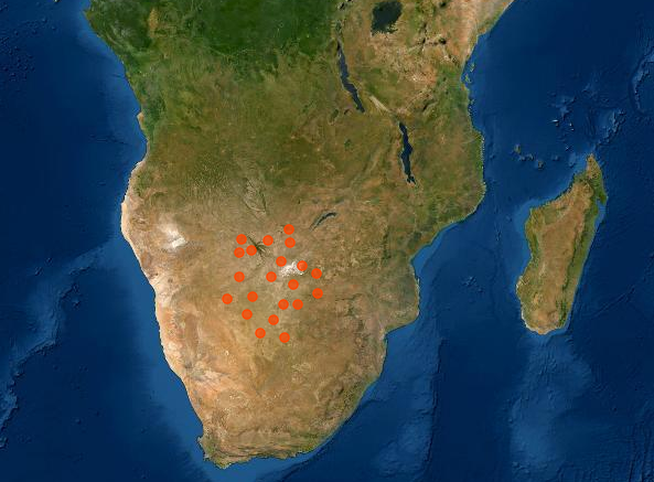
Here, we compute the array response function of a seismic array (NR) installed in Africa.
The Python method of computing ARF was implemented in get_relative_arf in the following codes.
 1
 2
 3
 4
 5
 6
 7
 8
 9
10
11
12
13
14
15
16
17
18
19
20
21
22
23
24
25
26
27
28
29
30
31
32
33
34
35
36
37
38
39
40
41
42
43
44
45
46
47
48
49
50
51
52
53
54
55
56
57
|
import numpy as np
import matplotlib.pyplot as plt
from geopy.distance import geodesic
from obspy.taup.taup_geo import calc_dist_azi as cda
from itertools import permutations
from scipy import interpolate

# Calculate ARF with relative coordinates.
def get_relative_arf(xy, f, b0=90, s0=0, s1=0, s2=5e-4, sn=51, bn=121):
    s = np.linspace(s1, s2, sn)
    b = np.linspace(0, 2*np.pi, bn)
    p = np.zeros((sn, bn), dtype=complex)
    n = len(xy)
    tmp = -2j * np.pi * f
    b00 = b0 / 180 * np.pi
    sl0 = np.array([-np.sin(b00), -np.cos(b00)]) * s0
    x0 = np.mean(xy[:, 0]); y0 = np.mean(xy[:, 1])
    pos = xy.copy(); pos[:, 0] -= x0; pos[:, 1] -= y0
    for i in range(sn):
        ss = s[i]
        for j in range(bn):
            bb = b[j]
            sl = np.array([-np.sin(bb), -np.cos(bb)]) * ss - sl0
            shift = sl[0] * pos[:, 0] + sl[1] * pos[:, 1]
            p[i, j] = np.sum(np.exp(tmp*shift))
    p = abs(p); p /= p.max(); p = 10 * np.log10(p**2)
    return b, s, p

# Plot array response function.
def plot_arf(xy, baz, slow, p):
    fig = plt.figure(figsize=(10, 4))
    fig.add_subplot(121)
    plt.scatter(xy[:, 0]/1e3, xy[:, 1]/1e3, s=200, marker='v',
                facecolor='b', edgecolor='k', lw=1.5, alpha=0.5)
    plt.xlabel('E-W (km)', fontsize=20)
    plt.ylabel('N-S (km)', fontsize=20)
    plt.xticks(fontsize=15)
    plt.yticks(fontsize=15)
    plt.grid(ls=(10, (8, 5)))
    plt.axis('equal')

    ax2 = fig.add_subplot(122, projection='polar')
    im = ax2.pcolormesh(baz, slow*1e3, p, cmap='magma',
                   vmin=-10, vmax=0)
    plt.xticks(fontsize=16)
    plt.yticks(fontsize=16)
    cbar = fig.colorbar(im, shrink=0.75, pad=0.13)
    cbar.set_label(r'Beam power (dB)', fontsize=15)
    cbar.ax.tick_params(labelsize=14)
    ax2.grid(color='gray', ls=(2, (10, 5)), lw=1)
    ax2.tick_params(axis='y', colors='c', labelsize=15, pad=15)
    ax2.set_theta_zero_location('N')
    ax2.set_theta_direction(-1)
    ax2.set_xlabel('Slowness (s/km)', fontsize=16)

    plt.tight_layout()
    plt.show()
|
A plane wave with slowness of 0 is given and we use formula $(1)$ to compute the ARF of NR :
 1
 2
 3
 4
 5
 6
 7
 8
 9
10
11
12
13
14
15
16
17
18
19
20
21
22
23
24
25
26
27
28
29
30
|
# Load geographical positions of seismic network and convert them to Cartesian system.
xy = []
with open('NR_NET.lst', 'r') as fin:
    for i, line in enumerate(fin.readlines()):
        tmp = line.strip().split('|')
        x = float(tmp[3]); y = float(tmp[2])
        if i < 1:
            xy.append([0., 0.])
            p0 = (y, x)
        else:
            p1 = (y, x)
            dist = geodesic(p1, p0, ellipsoid='WGS-84').km * 1e3
            _, az, _ = cda(p0[0], p0[1], p1[0], p1[1], 6371, 0)
            az = az / 180 * np.pi
            dx = dist * np.sin(az); dy = dist * np.cos(az)
            xy.append([dx, dy])
xy = np.array(xy)

# Parameter settings.
# Back-azimuth of plane wave source and corresponding slowness.
f = 0.02; b0 = 90; s0 = 0
# Scanning ranges of slowness.
s1 = 0; s2 = 5e-4
sn = 101; bn=  181
# Compute array response function spectra.
# Refrence position .
baz1, slow1, pow1 = get_relative_arf(xy, f, b0=b0, s0=s0, s1=s1, s2=s2, bn=bn, sn=sn)

# Visualization of ARF spectra.
plot_arf(xy, baz1, slow1, pow1)
|
1.2 The Improvement of the Resolution
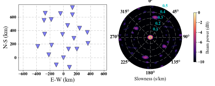
However, the above figure show a poor resolution of ARF, and the side lobes are not suppressed well. Thus, we need to improve the resolution and suppress the side lobes utilizing the cross positions instead of relative positions (Seismic Ambient Noise, edited by Nakata et al., 20019, page 35). The new ARF formula is given by
$$
ARF(\omega, \vec{s}, \vec{s}_0)= \frac{1}{N^2} \sum_{m=1}^N \sum_{n=1}^N \omega_m \omega_n e^{-i\omega(\vec{s}-\vec{s}_0)\cdot(\vec{r}_n-\vec{r}_m)} \tag{4}.
$$
The new version of ARF with cross positions is given by the following Python code.
 1
 2
 3
 4
 5
 6
 7
 8
 9
10
11
12
13
14
15
16
17
18
19
|
def get_cross_arf(xy, f, b0=90, s0=0, s1=0, s2=5e-4, sn=51, bn=121):
    b00 = b0 / 180 * np.pi
    s = np.linspace(s1, s2, sn)
    b = np.linspace(0, 2*np.pi, bn)
    tmp = -2j * np.pi * f
    n = len(xy[:, 0])
    p = np.zeros((sn, bn), dtype=complex)
    index = np.array(list(permutations(range(n), 2)))
    pos = xy[index[:, 1]] - xy[index[:, 0]]
    sl0 = np.array([-np.sin(b00), -np.cos(b00)]) * s0
    for i in range(sn):
        ss = s[i]
        for j in range(bn):
            bb = b[j]
            sl = np.array([-np.sin(bb), -np.cos(bb)]) * ss - sl0
            shift = sl[0] * pos[:, 0] + sl[1] * pos[:, 1]
            p[i, j] = np.sum(np.exp(tmp*shift))
    p = abs(p); p /= p.max(); p = 10 * np.log10(p**2)
    return b, s, p
|
We also use the NR network to compute its ARF.
1
2
3
|
# ARF of cross position.
baz2, slow2, pow2 = get_cross_arf(xy, f, b0=b0, s0=s0, s1=s1, s2=s2, bn=bn, sn=sn)
plot_arf(xy, baz2, slow2, pow2)
|
The above figure show a better resolution and the main lobe (where the slowness of the given plane wave is 0) is very clear.
2 Codes of Investigating the Array Configuration
 1
 2
 3
 4
 5
 6
 7
 8
 9
10
11
12
13
14
15
16
17
18
19
20
21
22
23
24
25
26
27
28
29
30
31
32
33
34
35
36
37
38
39
40
41
42
43
44
45
46
47
48
|
# Obtain ARF of given array geometry and parameters.
def get_arf(relative_pos, f, s1, s2, s0, b0, sn=51, bn=121):
    P = np.zeros((sn, bn), dtype=complex)
    slow = np.linspace(s1, s2, sn)
    baz = np.radians(np.linspace(0, 360, bn))
    b00 = np.radians(b0)
    for i, ss in enumerate(slow):
        for j, bb in enumerate(baz):
            shift = (-ss * np.sin(bb) + s0 * np.sin(b00)) * relative_pos[:, 0] +\
                    (-ss * np.cos(bb) + s0 * np.cos(b00)) * relative_pos[:, 1]
            P[i, j] = sum(np.exp(-1j * 2 * np.pi * f * shift))
    return baz, slow, P

# Visualization of ARF spectra.
def plot_spectra(baz, slow, p, b0, s0, coordinate, cmap='jet', figname='ARF_Example', savefig=False):
    PP = abs(p) ** 2
    bazz = baz.copy(); sloww = slow.copy()
    bazz = np.linspace(baz[0], baz[-1], 361)
    sloww = np.linspace(slow[0], slow[-1], 101)
    intp = interpolate.interp2d(baz, slow, PP, kind='cubic')
    PP = intp(bazz, sloww)
    PP = PP / PP.max()

    plt.figure(figsize=(12, 5))
    plt.subplot(121)
    plt.scatter(coordinate[:, 0], coordinate[:, 1], marker='v', s=300,
                facecolor='#87CEFA', edgecolor='k', linewidth=1.5)
    plt.xlabel('X (km)', fontsize=20)
    plt.ylabel('Y (km)', fontsize=20)
    plt.xticks(fontsize=15); plt.yticks(fontsize=15)
    plt.axis('equal'); plt.grid(color='gray', ls='--', lw=1.5)

    ax = plt.subplot(122, projection='polar')
    plt.pcolormesh(bazz, sloww*1e3, PP, cmap=cmap)
    cbar = plt.colorbar(shrink=0.75, pad=0.075)
    cbar.set_label(r'Normalized $\theta-S$ Spectra', fontsize=14)
    ax.grid(color='gray', ls='--', lw=2)
    ax.tick_params(axis='y', colors='#888888', labelsize=16, pad=15)
    ax.set_theta_zero_location('N')
    ax.set_theta_direction(-1)
    ax.plot(bazz, np.ones(len(bazz))*sloww.min()*1e3, c='k', lw=2)
    ax.plot(bazz, np.ones(len(bazz))*sloww.max()*1e3, c='k', lw=2)
    ax.scatter(b0/180*np.pi, s0*1e3, marker='+', s=150,
               facecolor='c', lw=3, zorder=10)
    ax.set_xlabel('Slowness (s/km)', fontsize=15)
    plt.xticks(fontsize=16)
    plt.tight_layout()
    plt.show()
|
3 Influence of the Array Configuration
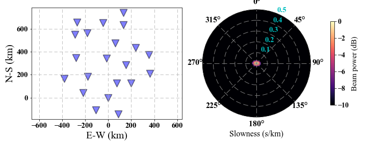
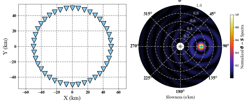
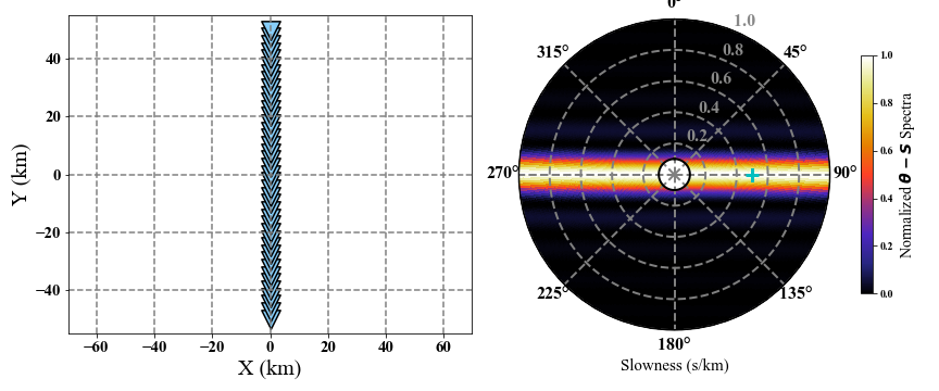
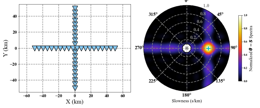
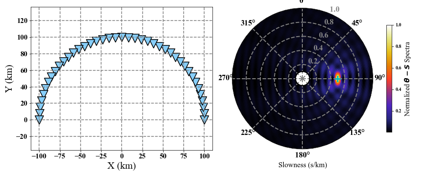
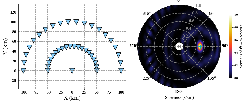
3.1 The geometry effects
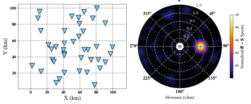
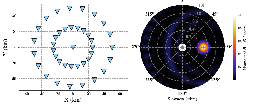
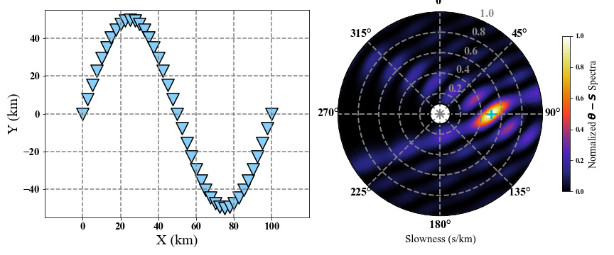
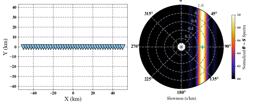
The geometry of the seismic array will control the back-azimuth independence of the plane wave signal. Bigger direction range can recognize the back-azimuth better.
 1
 2
 3
 4
 5
 6
 7
 8
 9
10
11
12
13
14
15
|
# Generate coordinates in km.
theta = np.linspace(0, 2*np.pi, 41); r = 50
coordinate = np.zeros((len(theta), 2))
coordinate[:, 0] = np.cos(theta) * r
coordinate[:, 1] = np.sin(theta) * r
# Parameter settings: in s/m
s1 = 1e-4; s2 = 1e-3
# The freaneucy.
f = 0.05
# The back-azimuth in degree and slowness in s/m of the given plane wave.
b0 = 90; s0 = 5e-4
# Obtain ARF spectra.
baz, slow, p = get_arf(coordinate*1e3, f, s1, s2, s0, b0, sn=51, bn=121)
# Interpolation and visualization.
plot_spectra(baz, slow, p, b0, s0, coordinate, cmap='CMRmap')
|
 1
 2
 3
 4
 5
 6
 7
 8
 9
10
11
12
|
# Generate random coordinates in km.
coordinate = np.random.random((41, 2)) * 100
# Parameter settings: in s/m
s1 = 1e-4; s2 = 1e-3
# The freaneucy.
f = 0.05
# The back-azimuth in degree and slowness in s/m of the given plane wave.
b0 = 90; s0 = 5e-4
# Obtain ARF spectra.
baz, slow, p = get_arf(coordinate*1e3, f, s1, s2, s0, b0, sn=51, bn=121)
# Interpolation and visualization.
plot_spectra(baz, slow, p, b0, s0, coordinate, cmap='CMRmap')
|
 1
 2
 3
 4
 5
 6
 7
 8
 9
10
11
12
13
14
15
16
17
18
19
|
# Generate coordinates in km.
coordinate = np.zeros((41, 2))
coordinate[20] = 0
theta = np.linspace(0, 2*np.pi, 20)
r1 = 25; r2 = 50
coordinate[:20, 0] = np.cos(theta) * r1
coordinate[:20, 1] = np.sin(theta) * r1
coordinate[21:, 0] = np.cos(theta) * r2
coordinate[21:, 1] = np.sin(theta) * r2
# Parameter settings: in s/m
s1 = 1e-4; s2 = 1e-3
# The freaneucy.
f = 0.05
# The back-azimuth in degree and slowness in s/m of the given plane wave.
b0 = 90; s0 = 5e-4
# Obtain ARF spectra.
baz, slow, p = get_arf(coordinate*1e3, f, s1, s2, s0, b0, sn=51, bn=121)
# Interpolation and visualization.
plot_spectra(baz, slow, p, b0, s0, coordinate, cmap='CMRmap')
|
 1
 2
 3
 4
 5
 6
 7
 8
 9
10
11
12
13
14
15
16
|
# Generate coordinates in km.
coordinate = np.zeros((41, 2))
theta = np.linspace(0, 2*np.pi, len(coordinate[:, 0]))
r = 100
coordinate[:, 0] = theta / abs(theta).max() * r
coordinate[:, 1] = np.sin(theta) * r / 2
# Parameter settings: in s/m
s1 = 1e-4; s2 = 1e-3
# The freaneucy.
f = 0.05
# The back-azimuth in degree and slowness in s/m of the given plane wave.
b0 = 90; s0 = 5e-4
# Obtain ARF spectra.
baz, slow, p = get_arf(coordinate*1e3, f, s1, s2, s0, b0, sn=51, bn=121)
# Interpolation and visualization.
plot_spectra(baz, slow, p, b0, s0, coordinate, cmap='CMRmap')
|
 1
 2
 3
 4
 5
 6
 7
 8
 9
10
11
12
13
14
15
|
# Generate coordinates in km.
coordinate = np.zeros((41, 2))
r = 100
coordinate[:, 0] = np.linspace(-r/2, r/2, len(coordinate[:, 0]))
coordinate[:, 1] = 0
# Parameter settings: in s/m
s1 = 1e-4; s2 = 1e-3
# The freaneucy.
f = 0.05
# The back-azimuth in degree and slowness in s/m of the given plane wave.
b0 = 90; s0 = 5e-4
# Obtain ARF spectra.
baz, slow, p = get_arf(coordinate*1e3, f, s1, s2, s0, b0, sn=51, bn=121)
# Interpolation and visualization.
plot_spectra(baz, slow, p, b0, s0, coordinate, cmap='CMRmap')
|
 1
 2
 3
 4
 5
 6
 7
 8
 9
10
11
12
13
14
15
|
# Generate coordinates in km.
coordinate = np.zeros((41, 2))
r = 100
coordinate[:, 1] = np.linspace(-r/2, r/2, len(coordinate[:, 1]))
coordinate[:, 0] = 0
# Parameter settings: in s/m
s1 = 1e-4; s2 = 1e-3
# The freaneucy.
f = 0.05
# The back-azimuth in degree and slowness in s/m of the given plane wave.
b0 = 90; s0 = 5e-4
# Obtain ARF spectra.
baz, slow, p = get_arf(coordinate*1e3, f, s1, s2, s0, b0, sn=51, bn=121)
# Interpolation and visualization.
plot_spectra(baz, slow, p, b0, s0, coordinate, cmap='CMRmap')
|
 1
 2
 3
 4
 5
 6
 7
 8
 9
10
11
12
13
14
15
16
17
|
# Generate coordinates in km.
coordinate = np.zeros((41, 2))
r = 100
coordinate[:21, 0] = 0
coordinate[:21, 1] = np.linspace(-r/2, r/2, 21)
coordinate[21:, 0] = np.linspace(-r/2, r/2, 20)
coordinate[21:, 1] = 0
# Parameter settings: in s/m
s1 = 1e-4; s2 = 1e-3
# The freaneucy.
f = 0.05
# The back-azimuth in degree and slowness in s/m of the given plane wave.
b0 = 90; s0 = 5e-4
# Obtain ARF spectra.
baz, slow, p = get_arf(coordinate*1e3, f, s1, s2, s0, b0, sn=51, bn=121)
# Interpolation and visualization.
plot_spectra(baz, slow, p, b0, s0, coordinate, cmap='CMRmap')
|
 1
 2
 3
 4
 5
 6
 7
 8
 9
10
11
12
13
14
15
16
|
# Generate coordinates in km.
coordinate = np.zeros((41, 2))
theta = np.linspace(0, np.pi, 41)
r = 100
coordinate[:, 0] = np.cos(theta) * r
coordinate[:, 1] = np.sin(theta) * r
# Parameter settings: in s/m
s1 = 1e-4; s2 = 1e-3
# The freaneucy.
f = 0.05
# The back-azimuth in degree and slowness in s/m of the given plane wave.
b0 = 90; s0 = 5e-4
# Obtain ARF spectra.
baz, slow, p = get_arf(coordinate*1e3, f, s1, s2, s0, b0, sn=51, bn=121)
# Interpolation and visualization.
plot_spectra(baz, slow, p, b0, s0, coordinate, cmap='CMRmap')
|
 1
 2
 3
 4
 5
 6
 7
 8
 9
10
11
12
13
14
15
16
17
18
19
|
# Generate coordinates in km.
coordinate = np.zeros((41, 2))
theta = np.linspace(0, np.pi, 20)
r1 = 50; r2 = 100
coordinate[:20, 0] = np.cos(theta) * r1
coordinate[:20, 1] = np.sin(theta) * r1
theta = np.linspace(0, np.pi, 20)
coordinate[21:, 0] = np.cos(theta) * r2
coordinate[21:, 1] = np.sin(theta) * r2
# Parameter settings: in s/m
s1 = 1e-4; s2 = 1e-3
# The freaneucy.
f = 0.05
# The back-azimuth in degree and slowness in s/m of the given plane wave.
b0 = 90; s0 = 5e-4
# Obtain ARF spectra.
baz, slow, p = get_arf(coordinate*1e3, f, s1, s2, s0, b0, sn=51, bn=121)
# Interpolation and visualization.
plot_spectra(baz, slow, p, b0, s0, coordinate, cmap='CMRmap')
|
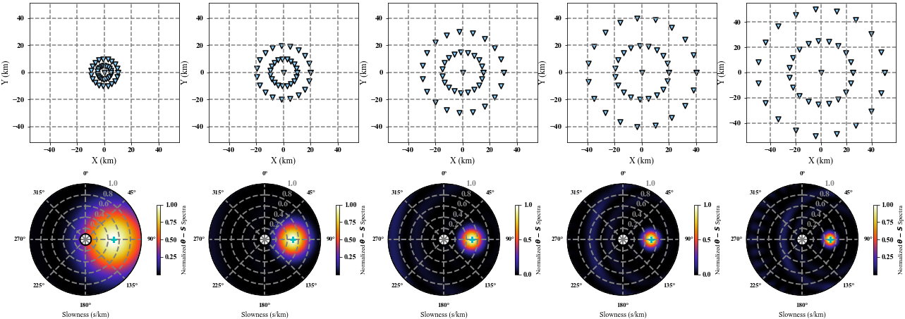
3.2 The aperture of the array
The aperture of seismic array defines the resolution and we show that the bigger aperture, the higher resolution will be obtained. Here, we give a plane wave with frequency of $0.05 Hz$, slowness of $5e^{-4} s/m$ and back-azimuth of $90 ^o$.
 1
 2
 3
 4
 5
 6
 7
 8
 9
10
11
12
13
14
15
16
17
18
19
20
21
22
23
24
25
26
27
28
29
30
31
32
33
34
35
36
37
38
39
40
41
42
43
44
45
46
47
48
49
50
51
52
53
|
# Parameter settings: in s/m
s1 = 1e-4; s2 = 1e-3
# The freaneucy.
f = 0.05
# The back-azimuth in degree and slowness in s/m of the given plane wave.
b0 = 90; s0 = 5e-4

plt.figure(figsize=(22, 8))
for i in range(5):
    # Generate coordinates in km.
    coordinate = np.zeros((41, 2))
    coordinate[20] = 0
    theta = np.linspace(0, 2*np.pi, 20)
    r1 = 5*(i+1); r2 = 2 * r1
    coordinate[:20, 0] = np.cos(theta) * r1
    coordinate[:20, 1] = np.sin(theta) * r1
    coordinate[21:, 0] = np.cos(theta) * r2
    coordinate[21:, 1] = np.sin(theta) * r2

    # Obtain ARF spectra.
    baz, slow, P = get_arf(coordinate*1e3, f, s1, s2, s0, b0, sn=51, bn=121)
    PP = abs(P) ** 2
    bazz = baz.copy(); sloww = slow.copy()
    bazz = np.linspace(baz[0], baz[-1], 361)
    sloww = np.linspace(slow[0], slow[-1], 101)
    intp = interpolate.interp2d(baz, slow, PP, kind='cubic')
    PP = intp(bazz, sloww)
    PP = PP / PP.max()

    plt.subplot(2, 5, i+1)
    plt.scatter(coordinate[:, 0], coordinate[:, 1], marker='v', s=50,
                facecolor='#87CEFA', edgecolor='k', linewidth=1.5)
    plt.xlabel('X (km)', fontsize=12)
    plt.ylabel('Y (km)', fontsize=12)
    plt.xticks(fontsize=11); plt.yticks(fontsize=11)
    plt.axis('equal'); plt.grid(color='gray', ls='--', lw=1.5)
    plt.xlim(-55, 55); plt.ylim(-55, 55)

    ax = plt.subplot(2, 5, i+6, projection='polar')
    plt.pcolormesh(bazz, sloww*1e3, PP, cmap='CMRmap')
    cbar = plt.colorbar(shrink=0.5, pad=0.1)
    cbar.set_label(r'Normalized $\theta-S$ Spectra', fontsize=9)
    ax.grid(color='gray', ls='--', lw=2)
    ax.tick_params(axis='y', colors='#888888', labelsize=12, pad=10)
    ax.set_theta_zero_location('N')
    ax.set_theta_direction(-1)
    ax.plot(bazz, np.ones(len(bazz))*sloww.min()*1e3, c='k', lw=2)
    ax.plot(bazz, np.ones(len(bazz))*sloww.max()*1e3, c='k', lw=2)
    ax.scatter(b0/180*np.pi, s0*1e3, marker='+', s=75,
               facecolor='c', lw=3, zorder=10)
    ax.set_xlabel('Slowness (s/km)', fontsize=10)
    plt.xticks(fontsize=9)
plt.show()
|
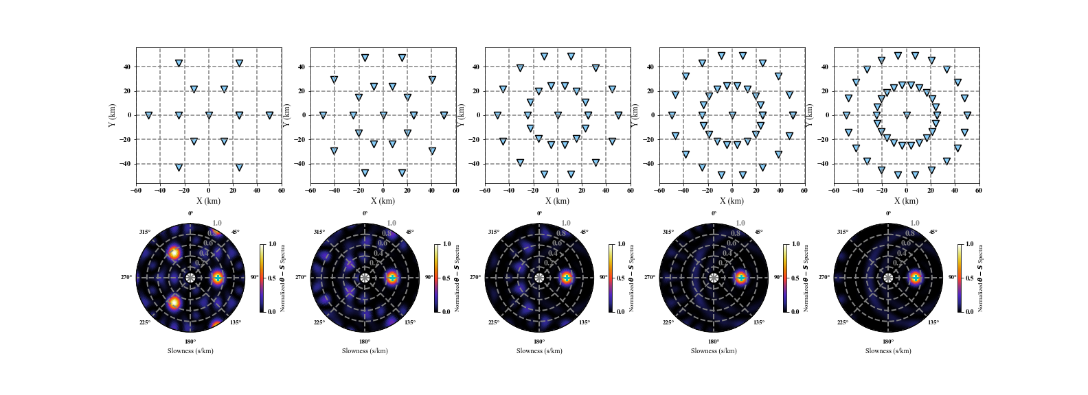
3.3 The number of receivers
In general, more receivers in the array will improve the quality of scanning the coherent plane wave signal. Here, we compare the ARF results from different arrays composed of i incremental receivers.
 1
 2
 3
 4
 5
 6
 7
 8
 9
10
11
12
13
14
15
16
17
18
19
20
21
22
23
24
25
26
27
28
29
30
31
32
33
34
35
36
37
38
39
40
41
42
43
44
45
46
47
48
49
50
51
52
53
54
55
|
# Parameter settings: in s/m
s1 = 1e-4; s2 = 1e-3
# The freaneucy.
f = 0.05
# The back-azimuth in degree and slowness in s/m of the given plane wave.
b0 = 90; s0 = 5e-4
# The radia in km of the two circles.
r1 = 25; r2 = 50

plt.figure(figsize=(22, 8))
for i in range(5):
    # Generate coordinates in km.
    coordinate = np.zeros((15+8*i, 2))
    n = len(coordinate[:, 0]); hn = n // 2
    coordinate[hn] = 0
    theta = np.linspace(0, 2*np.pi, hn)
    coordinate[:hn, 0] = np.cos(theta) * r1
    coordinate[:hn, 1] = np.sin(theta) * r1
    coordinate[hn+1:, 0] = np.cos(theta) * r2
    coordinate[hn+1:, 1] = np.sin(theta) * r2

    # Obtain ARF spectra.
    baz, slow, P = get_arf(coordinate*1e3, f, s1, s2, s0, b0, sn=51, bn=121)
    PP = abs(P) ** 2
    bazz = baz.copy(); sloww = slow.copy()
    bazz = np.linspace(baz[0], baz[-1], 361)
    sloww = np.linspace(slow[0], slow[-1], 101)
    intp = interpolate.interp2d(baz, slow, PP, kind='cubic')
    PP = intp(bazz, sloww)
    PP = PP / PP.max()

    plt.subplot(2, 5, i+1)
    plt.scatter(coordinate[:, 0], coordinate[:, 1], marker='v', s=100,
                facecolor='#87CEFA', edgecolor='k', linewidth=1.5)
    plt.xlabel('X (km)', fontsize=12)
    plt.ylabel('Y (km)', fontsize=12)
    plt.xticks(fontsize=11); plt.yticks(fontsize=11)
    plt.axis('equal'); plt.grid(color='gray', ls='--', lw=1.5)
    plt.xlim(-60, 60); plt.ylim(-60, 60)

    ax = plt.subplot(2, 5, i+6, projection='polar')
    plt.pcolormesh(bazz, sloww*1e3, PP, cmap='CMRmap')
    cbar = plt.colorbar(shrink=0.5, pad=0.1)
    cbar.set_label(r'Normalized $\theta-S$ Spectra', fontsize=9)
    ax.grid(color='gray', ls='--', lw=2)
    ax.tick_params(axis='y', colors='#888888', labelsize=12, pad=10)
    ax.set_theta_zero_location('N')
    ax.set_theta_direction(-1)
    ax.plot(bazz, np.ones(len(bazz))*sloww.min()*1e3, c='k', lw=2)
    ax.plot(bazz, np.ones(len(bazz))*sloww.max()*1e3, c='k', lw=2)
    ax.scatter(b0/180*np.pi, s0*1e3, marker='+', s=75,
               facecolor='c', lw=3, zorder=10)
    ax.set_xlabel('Slowness (s/km)', fontsize=10)
    plt.xticks(fontsize=9)
plt.show()
|
Bibliography
Johannes Schweitzer, Jan Fyen, Svein Mykkeltveit, Steven J. Gibbons, Myrto Pirli, Daniela Kühn, and Tormod Kværna 2011 Seismic Array Chapter 9.
Nakata, N. , Gualtieri, L. , & Fichtner, A. . (2019). Seismic Ambient Noise. P. 35.
