1 Introduction
The Bessel functions of the first kind can be defined by the series,
$$
J_{n}(x)=(\frac{x}{2})^n\sum_{k=0}^{\infty}\frac{(-\frac{x^2}{4})^k}{k!\Gamma(n+k+1)} \tag{1},
$$
where, $\Gamma(n+k+1)=(n+k)!$ when $n$ is an integer. However, the Bessel functions are difficult to directly calculate, so the numerical approximations are taken into consideration to obtain their values. Here, we show that how to utilize asymptotic expressions or polynomials to compute the numerical approximations of Bessel functions.
2 Numerical approximations
2.1 Simple approximation
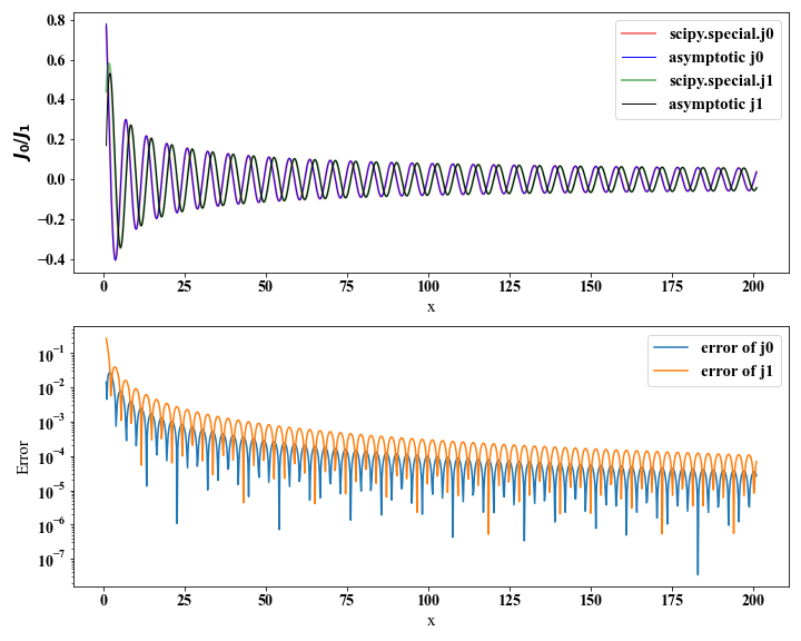
We first consider $J_n (x)$, and it looks like sine or cosine function with amplitude decaying as $x^{-1/2}$. When $x \gg n$. the asymptotic forms of $J_n(x)$ are defined as
$$
J_n(x) \sim \sqrt{\frac{2}{\pi x}} cos(x-\frac{1}{2}n x-\frac{\pi}{4}) \tag{2}.
$$
Specially, we have
$$
J_0(x) \sim \sqrt{\frac{2}{\pi x}}cos(x-\frac{\pi}{4}) \tag{3}
$$
with $x>0$.
Here, we compare the results from scipy.special and $(3)$, respectively.
 1
 2
 3
 4
 5
 6
 7
 8
 9
10
11
12
13
14
15
16
17
18
19
20
21
22
23
24
25
26
27
28
29
30
31
32
|
import numpy as np
import matplotlib.pyplot as plt
from scipy.special import j0, j1, i0

x0 = 1
x = np.linspace(x0, x0+200, 1001)
d11 = j0(x)
d21 = j1(x)
n = 0
d12 = (2/np.pi/x)**0.5 * np.cos(x-n*np.pi/2-np.pi/4)
n = 1
d22 = (2/np.pi/x)**0.5 * np.cos(x-n*np.pi/2-np.pi/4)

plt.figure(figsize=(10, 8))
plt.subplot(211)
plt.plot(x, d11, lw=2, color='r', alpha=0.5, label='scipy.speciall.j0')
plt.plot(x, d12, lw=1, color='b',label='asymptotic j0')
plt.plot(x, d21, lw=2, color='g', alpha=0.5,  label='scipy.speciall.j0')
plt.plot(x, d22, lw=1, color='k', label='asymptotic j0')
plt.legend(fontsize=15, loc='upper right')
plt.xlabel('x', fontsize=15)
plt.ylabel('$J_0$', fontsize=15)
plt.xticks(fontsize=14); plt.yticks(fontsize=14)
plt.subplot(212)
plt.semilogy(x, abs(d11-d12), lw=1.5, label='error of j0')
plt.semilogy(x, abs(d21-d22), lw=1.5, label='error of j1')
plt.legend(fontsize=15, loc='upper right')
plt.xlabel('x', fontsize=15)
plt.ylabel('Error', fontsize=15)
plt.xticks(fontsize=14); plt.yticks(fontsize=14)
plt.tight_layout()
plt.show
|
The Bessel functions have the following recurrence relation,
$$
J_{n+1}(x)=\frac{2n}{x}J_n(x)-J_{n-1}(x) \tag{4},
$$
so we can obtain Bessel functions with higher orders using recurrence formula $(4)$.
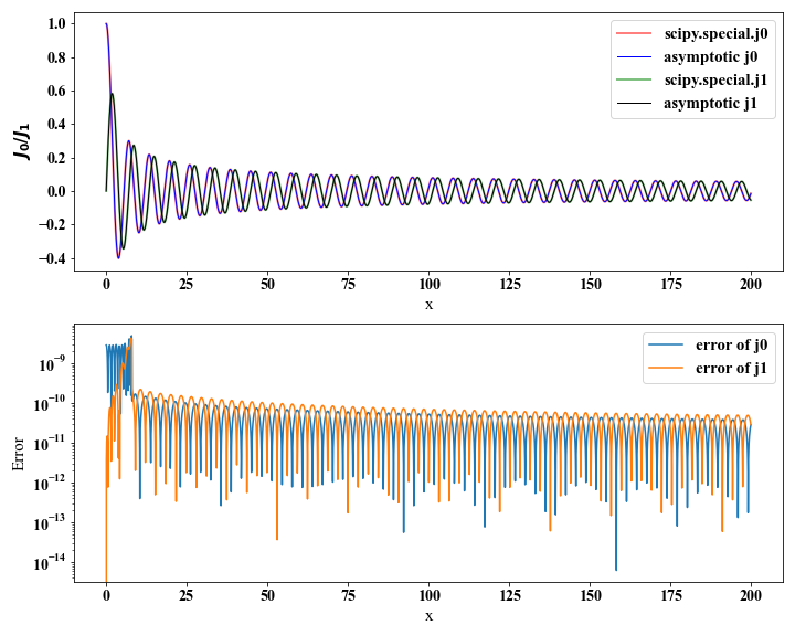
2.2 More precise approximation
For obtaining more precise values of Bessel functions, we should consider more polynomials. Here, we directly give the code of approximating the Bessel functions.
 1
 2
 3
 4
 5
 6
 7
 8
 9
10
11
12
13
14
15
16
17
18
19
20
21
22
23
24
25
26
27
28
29
30
31
32
33
34
35
36
37
38
39
40
41
42
43
44
45
|
# J0(x)
def bess_j0(x):
    ans = np.zeros_like(x)
    for i, ax in enumerate(x):
        if ax < 8:
            y= ax * ax
            ans1 = 57568490574.0+y*(-13362590354.0+y*(651619640.7
            +y*(-11214424.18+y*(77392.33017+y*(-184.9052456)))))
            ans2 = 57568490411.0+y*(1029532985.0+y*(9494680.718
            +y*(59272.64853+y*(267.8532712+y*1.0))))
            ans[i] = ans1 / ans2
        else:
            z=8/ax
            y=z*z;
            xx=ax-0.785398164;
            ans1=1.0+y*(-0.1098628627e-2+y*(0.2734510407e-4
            +y*(-0.2073370639e-5+y*0.2093887211e-6)))
            ans2 = -0.1562499995e-1+y*(0.1430488765e-3
            +y*(-0.6911147651e-5+y*(0.7621095161e-6
            -y*0.934945152e-7)))
            ans[i] = np.sqrt(0.636619772/ax)*(np.cos(xx)*ans1-z*np.sin(xx)*ans2)
    return ans

# J1(x)
def bess_j1(x):
    ans = np.zeros_like(x)
    for i, ax in enumerate(x):
        if ax < 8:
            y = ax * ax
            ans1 = ax * (72362614232.0 + y*(-7895059235.0 + y*(242396853.1
                 + y*(-2972611.439 + y*(15704.48260 + y*(-30.16036606))))))
            ans2 = 144725228442.0+y*(2300535178.0+y*(18583304.74
            +y*(99447.43394+y*(376.9991397+y*1.0))))
            ans[i] = ans1 / ans2
        else:
            z = 8.0/ax
            y = z*z
            xx = ax-2.356194491;
            ans1 = 1.0+y*(0.183105e-2+y*(-0.3516396496e-4
            +y*(0.2457520174e-5+y*(-0.240337019e-6))))
            ans2 = 0.04687499995+y*(-0.2002690873e-3
            +y*(0.8449199096e-5+y*(-0.88228987e-6
            +y*0.105787412e-6)))
            ans[i] = np.sqrt(0.636619772/ax)*(np.cos(xx)*ans1-z*np.sin(xx)*ans2)
    return ans
|
The results separately from scipy.special and polynomials are shown in the following figure.
 1
 2
 3
 4
 5
 6
 7
 8
 9
10
11
12
13
14
15
16
17
18
19
20
21
22
23
24
25
|
x = np.linspace(0, 200, 4001)
d11 = j0(x)
d21 = j1(x)
d12 = bess_j0(x)
d22 = bess_j1(x)

plt.figure(figsize=(10, 8))
plt.subplot(211)
plt.plot(x, d11, lw=2, color='r', alpha=0.5, label='scipy.speciall.j0')
plt.plot(x, d12, lw=1, color='b',label='asymptotic j0')
plt.plot(x, d21, lw=2, color='g', alpha=0.5,  label='scipy.speciall.j0')
plt.plot(x, d22, lw=1, color='k', label='asymptotic j0')
plt.legend(fontsize=15, loc='upper right')
plt.xlabel('x', fontsize=15)
plt.ylabel('$J_0$', fontsize=15)
plt.xticks(fontsize=14); plt.yticks(fontsize=14)
plt.subplot(212)
plt.semilogy(x, abs(d11-d12), lw=1.5, label='error of j0')
plt.semilogy(x, abs(d21-d22), lw=1.5, label='error of j1')
plt.legend(fontsize=15, loc='upper right')
plt.xlabel('x', fontsize=15)
plt.ylabel('Error', fontsize=15)
plt.xticks(fontsize=14); plt.yticks(fontsize=14)
plt.tight_layout()
plt.show
|
Bibliography
Press, W. H. , Flannery, B. P. , Teukolsky, S. A. , & Vetterling, W. T. . (1988). Numerical recipes in c: the art of scientific computing.
