1 Basic Principles
The Multi-Channel Analysis of Surface Waves (MASW) is very popular in the past over two decades and the estimations of shear wave velocity models have benefited much from MASW in civil engineering field (Park et al., 1998). Here we simply introduce the basic principles of MASW. Assume that we obtain seismic records of surface waves $ u(t, x) $, and the frequency-phase velocity spectra is given by
$$
\begin{aligned}
P(\omega, c) &=\int_0^\infty \frac{U(\omega, x)}{|U(\omega, x)|}e^{i k x }dx \\
&= \int_0^\infty \frac{U(\omega, x)}{|U(\omega, x)|}e^{i \frac{\omega}{c} x }dx
\end{aligned} \tag{1},
$$
where, $k$ is wave number, $\omega$ is angular frequency, $c$ is phase velocity, and $U(\omega, x)$ is the Fourier spectrum of record $u(t, x)$ at offset $x$. In realistic applications, however, the time and space is discrete, and we rewrite $(1)$ as
$$
P(\omega, c)=\sum_{n=1}^N\frac{U(\omega, x_n)}{|U(\omega, x_n)|}e^{i\frac{\omega}{c}x_n}\Delta x \tag{2},
$$
where, $N$ is the total number of channels.
2 Examples
2.1 Python code
Here, we give a very simple code demo of implementing MASW.
 1
 2
 3
 4
 5
 6
 7
 8
 9
10
11
12
13
14
15
16
17
|
def masw_fc_trans(data, dt, dist, f1, f2, c1, c2, nc=201):
    m, n = data.shape
    fs = 1 / dt; fn1 = int(f1*n/fs); fn2 = int(f2*n/fs)
    c = np.linspace(c1, c2, nc)
    f = np.arange(n) * fs / (n-1)
    df = f[1] - f[0]
    w = 2 * np.pi * f
    fft_d = np.zeros((m, n), dtype=np.complex)
    for i in range(m):
    	fft_d[i] = np.fft.fft(data[i])
    fft_d = fft_d / abs(fft_d)
    fft_d[np.isnan(fft_d)] = 0
    fc = np.zeros((len(c), len(w[fn1: fn2+1])))
    for ci, cc in enumerate(c):
        for fi in range(fn1, fn2+1) :
            fc[ci, fi-fn1] = abs(sum(np.exp(1j*w[fi]/cc*dist)*fft_d[:, fi]))
    return f[fn1: fn2+1], c, fc/abs(fc).max()
|
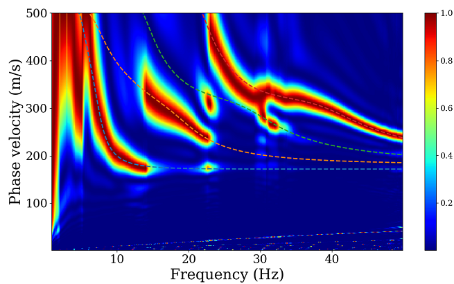
2.2 Frequency-phase velocity spectra
We computed synthetic vertical-component traces using the CPS330 package (Herrmann, 2013, http://www.eas.slu.edu/eqc/eqccps.html) based on a multi-layered model. Four modes of Rayleigh waves in total have been taken into consideration to synthesize seismic traces. We use MASW method to retrieve dispersion curves of Rayleigh waves from these synthetic seismic traces. Synthetic seismic traces and corresponding dispersion curves can be obtained from https://github.com/geophydog/Seismic_Data_Examples/tree/main/MASW_Traces_x1_10m_dx_1m.
 1
 2
 3
 4
 5
 6
 7
 8
 9
10
11
12
13
14
15
16
17
18
19
20
21
22
23
24
25
26
27
28
29
30
31
32
33
34
35
36
37
38
39
40
41
42
43
44
45
46
47
48
49
50
51
52
53
54
55
|
import numpy as np
from scipy import fft
import sys
import matplotlib.pyplot as plt
from obspy import read

def main():
    # Offset begins at 10 m and the interval is 1 m.
    x1 = 10; dx = 1
    # Read in masw seismic traces.
    # You can download the data sets from  "https://github.com/geophydog/Seismic_Data_Examples/tree/main/MASW_Traces_x1_10m_dx_1m".
    st = read('*Z00.sac')
    data = []
    for i, tr in enumerate(st):
        d = tr.data; d /= abs(d).max()
        data.append(d)
    data = np.array(data)
    dist = x1 + np.arange(len(st)) * dx
    # Parameters settings.
    f1 = 1; f2 = 50; c1 = 1; c2 = 500; nc = 500
    dt = tr.stats.delta
    # Call masw transform to obtain f-c spectra.
    f, c, p = masw_fc_trans(data, dt, dist, f1, f2, c1, c2, nc=nc)
    # Plot the f-c spectra.
    # File "SREGN.TXT" can also be downloaded from "https://github.com/geophydog/Seismic_Data_Examples/tree/main/MASW_Traces_x1_10m_dx_1m".
    ds = {}
    with open(r'SREGN.TXT', 'r') as fin:
        lines = fin.readlines()
        for i, line in enumerate(lines):
            s = line.strip().split()
            if len(s) > 7 and s[6] == 'GAMMA' and s[7] == 'ELP':
                if len(ds.keys()) > 0:
                    ds[mode] = np.array(ds[mode])
                tmp = lines[i-1].split()
                mode = tmp[2] + tmp[4]
                ds[mode] = []
            if len(s) > 7 and s[0].isdigit():
                ds[mode].append([float(s[2]), float(s[3])])
    ds[mode] = np.array(ds[mode])
    for i in range(len(p[0])):
        p[:, i] /= p[:, i].max()
    plt.figure(figsize=(7,5))
    plt.pcolormesh(f, c, p**2, cmap='jet')
    plt.colorbar()
    for k in ds.keys():
        dc = ds[k]
        plt.plot(dc[:, 0], dc[:, 1]*1e3, '--', lw=2)
    plt.xlabel('Frequency (Hz)', fontsize=25)
    plt.ylabel('Phase velocity (m/s)', fontsize=25)
    plt.xticks(fontsize=20)
    plt.yticks(fontsize=20)
    plt.xlim(f[0], f[-1])
    plt.ylim(c[0], c[-1])
    plt.tight_layout()
    plt.show()
|
3 Bibliography
Park, C. B., Miller, R. D., & Xia, J. (1998). Imaging dispersion curves of surface waves on
multi-channel record. Seg Technical Program Expanded Abstracts, 1377–1380.
Herrmann, R. B. (2013). Computer programs in seismology: An evolving tool for instruction
and research. Seismological Research Letters, 84(6), 1081–1088.
