Hilbert Transform

Firstly, compute the FFT of real signal $x(n)$ $$ X(k) = \mathscr{F}[x(n)]=\sum_{n=0}^{N-1}x(n)e^{-\frac{i2\pi kn}{N}} \tag{1}. $$

Let the FFT of $h(n)$ be $H(k)$ to yield
$$ H(k)= \begin{cases} &X(k), &\text{ for } k=0 \\
&2X(k), &\text{ for } k=1, 2, \cdots, \frac{N}{2}-1 \\
&0, &\text{ for } k=\frac{N}{2}, \frac{N}{2}+1,\cdots, N-1 \end{cases} \tag{2}. $$

The hilbert transform $h(n)$ of the real signal $x(n)$ is given by
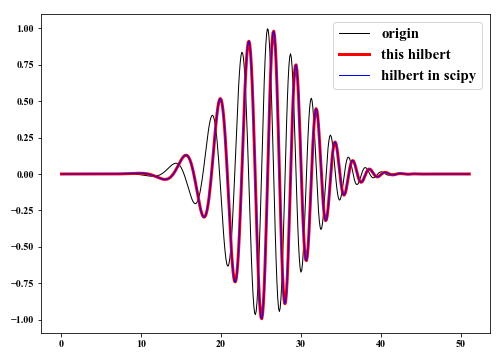
$$ h(n) = \mathscr{I} \{ \mathscr{F}^{-1}[H(k)] \} \tag{3}. $$ $h(n)$ and $x(n)$ are the imaginary and real parts of signals, respectively. Here, we implement the $Hilbert \ transform$ using Python and compare it with that computed with $hiltert$ method in $scipy.signal$.

 1
 2
 3
 4
 5
 6
 7
 8
 9
10
11
12
13
14
15
16
17
18
19
20
21
22
23

import numpy as np
import matplotlib.pyplot as plt
from scipy.signal import hilbert

n = 512
dt = 0.1
t = np.arange(n) * dt

x = np.sin(t**2/25) * np.exp(-(t-t[n//2])**2/50)
fx = np.fft.fft(x)
fh = fx.copy()
fh[1: n//2] = 2 * fx[1: n//2]
fh[n//2:] = 0
h1 = np.fft.ifft(fh).imag
h2 = hilbert(x).imag

plt.figure(figsize=(10, 6))
plt.plot(t, x, 'k', lw=1, label='origin')
plt.plot(t, h1, 'r', lw=3, label='this hilbert')
plt.plot(t, h2, 'b', lw=1, label='hilbert in scipy')
plt.legend(fontsize=15)
plt.tight_layout()
plt.show()

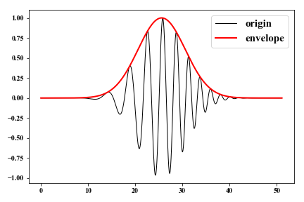
The envelope of a signal can be calculated using $Hilbert \ transform$ with
$$ E(n) =\sqrt{x^2(n)+h^2(n)} \tag{4}. $$

1
2
3
4
5
6
7

e = (x**2+h1**2) ** 0.5
plt.figure(figsize=(8, 5))
plt.plot(t, x, 'k', lw=1, label='origin')
plt.plot(t, e, 'r', lw=2, label='envelope')
plt.legend(fontsize=15)
plt.tight_layout()
plt.show()