1 Background

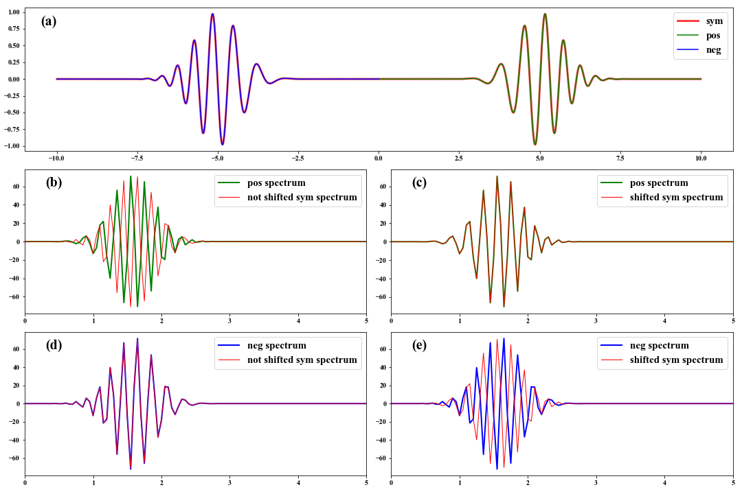
Ambient seismic noise cross-correlation has far-reaching implications for the passive seismic surface wave imaging from regional to continental scales (e.g. Campillo & Paul, Shapiro & Campillo, 2004). Spectral analysis of cross-correlations is the key to retrieving reliable dispersion information about surface waves. Based on the Fourier spectra of event seismic surface wave data, however, we need to shift the cross-correlation time function before doing FFT to obtain the right spectra.

2 A numerical example

Here, we generate a linear frequency modulated signal with decaying as $e^{-(t-t0)^2}$, and create a symmetric signal like cross-correlation functions extracted from seismic noise. The Fourier spectra separately from shifted and not shifted symmetric signal will be compared with the spectra of the positive and negative signals.

 1
 2
 3
 4
 5
 6
 7
 8
 9
10
11
12
13
14
15
16
17
18
19
20
21
22
23
24
25
26
27
28
29
30
31
32
33
34
35
36
37
38
39
40
41
42
43
44
45
46
47
48
49
n = 1001; nn = 2 * n - 1
t = np.linspace(0, 10, n)
s = np.sin(t**2) * np.exp(-(t-5)**2)
ss = np.zeros(nn)
ss[:n] = s[::-1]; ss[n-1:] = s
tt = np.linspace(-10, 10, len(ss))
f = np.arange(nn) / (t[1]-t[0]) / (nn-1)
fd1 = np.fft.fft(s, nn)
fd2 = np.fft.fft(s[::-1], nn)
fdd1 = np.fft.fft(ss, nn) / 2
fdd2 = np.fft.fft(np.fft.fftshift(ss), nn) / 2

plt.figure(figsize=(15, 10))
plt.subplot(311)
plt.plot(tt, ss, lw=3, color='r', alpha=0.75, label='sym')
plt.plot(t, s, lw=1.5, color='g', label='pos')
plt.plot(-t[::-1], s[::-1], lw=1.5, color='b', label='neg')
plt.text(-10.5, 0.8, '(a)', fontdict={'size':20})

plt.legend(fontsize=15, loc='upper right')

plt.subplot(323)
plt.plot(f, fd1.real, lw=2, color='g', label='pos spectrum')
plt.plot(f, fdd1.real, lw=1, color='r', label='not shifted sym spectrum')
plt.legend(fontsize=15, loc='upper right')
plt.text(0.3, 60, '(b)', fontdict={'size':20})
plt.xlim(0, 5)

plt.subplot(324)
plt.plot(f, fd1.real, lw=2, color='g', label='pos spectrum')
plt.plot(f, fdd2.real, lw=1, color='r', label='shifted sym spectrum')
plt.legend(fontsize=15, loc='upper right')
plt.text(0.3, 60, '(c)', fontdict={'size':20})
plt.xlim(0, 5)

plt.subplot(325)
plt.plot(f, fd2.real, lw=2, color='b', label='neg spectrum')
plt.plot(f, fdd1.real, lw=1, color='r', label='not shifted sym spectrum')
plt.legend(fontsize=15, loc='upper right')
plt.text(0.3, 60, '(d)', fontdict={'size':20})
plt.xlim(0, 5)

plt.subplot(326)
plt.plot(f, fd2.real, lw=2, color='b', label='neg spectrum')
plt.plot(f, fdd2.real, lw=1, color='r', label='shifted sym spectrum')
plt.legend(fontsize=15, loc='upper right')
plt.text(0.3, 60, '(e)', fontdict={'size':20})
plt.xlim(0, 5)
plt.show()

CCF_Spectra

Bibliography

Campillo, M., & Paul, A. (2003). Long-range correlations in the diffuse seismic coda. Science, 299(5606), 547–549.

Shapiro, N. M., & Campillo, M. (2004). Emergence of broadband rayleigh waves from correlations of the ambient seismic noise. Geophysical Research Letters, 31(7).