1 Acoustic wave equation
The acoustic wave equation in vector form is given by
$$
p_{tt}=c^2 \nabla^2 p \tag{1}
$$
where, $p$ is the acoustic pressure, $c$ is the propagation speed of
acoustic wave, $p_{tt}$ is the second time derivative of $p$,
and $\nabla^2$ denotes the $Laplacian$ operator. We will discretize
the equation using finite difference method in the following parts.
2 Propagation in 1D space
The Taylar’s series of $p(t+\Delta t)$ and $p(t-\Delta t)$ are given by
$$
\left \{
\begin{aligned}
p(t+\Delta t) &= p(t) + p’(t)\Delta t + \frac{1}{2}p’'(t)\Delta t^2 + \mathcal{O}(\Delta t^2)\\
p(t-\Delta t) &= p(t) - p’(t)\Delta t + \frac{1}{2}p’'(t)\Delta t^2 + \mathcal{O}(\Delta t^2)
\end{aligned}
\right. \tag{2},
$$
so we get $p_{tt}$ in discrete form as
$$
p_{tt}=\frac{\partial ^2 p(x, t)}{\partial t^2}=
\frac{p(x, t+\Delta t)-2p(x, t)+p(x, t-\Delta t)}{\Delta t^2} \tag{3}.
$$
Similarly, the discretae form of $\nabla^2p$ becomes
$$
\nabla^2 p = \frac{p(x+\Delta x)-2p(x)+p(x-\Delta x)}{\Delta x^2} \tag{4}.
$$
Lastly, we get the 3-point finite difference in time and space domains of 1D acoustic wave
and the updated pressure is given by
$$
\begin{aligned}
p(x, t+\Delta t) &= 2p(x, t) - p(x, t-\Delta t)\\
&+ \frac{c^2\Delta t^2}{\Delta x^2}[p(x+\Delta x, t)-2p(x, t)+p(x-\Delta x, t)]
\end{aligned} \tag{5}.
$$
For simplicity, we rewrite eq. (5) as
$$
p^{i+1}_j = 2p^i_j-p^{i-1}_j + \frac{c^2\Delta t^2}{\Delta x^2}[p^i_{j+1}-2p^i_j+p^i_{j-1}] \tag{6},
$$
where, $i, j$ indicate the indices of time and space, respectively.
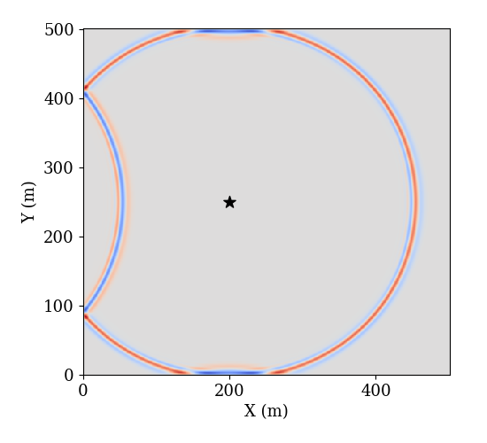
3 Propagation in 2D space
For the acoustic wave in 2D homogenous space domains, we have
$$
\frac{\partial ^2p(x, t)}{\partial t^2} = c^2
[\frac{\partial ^2p(x, t)}{\partial x^2} + \frac{\partial ^2p(x, t)}{\partial y^2}] \tag{7}.
$$
Here, we use $i, j, k$ to indicate the indices of time, $x$ and $y$, respectively. Thus,
$$
p^{i+1}_{j, k}=2p^i_{i, j}-p^{i-1}_{j,k}+c^2\Delta t^2
[\frac{p^i_{j, k+1}-2p^i_{j,k}+p^i_{j,k-1}}{\Delta x^2}+
\frac{p^i_{j+1, k}-2p^i_{j,k}+p^i_{j-1,k}}{\Delta y^2}+
] \tag{8}.
$$
4 Stability condition
$$
\frac{c \Delta t}{\Delta x} \le 1 \tag{9}.
$$
5 Numerical examples
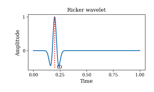
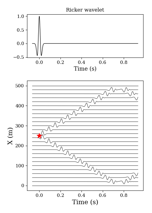
We use Ricker wavelet as the excitation of the acoustic wave equation,
and the Ricker wavelet is given by
$$
r(t)=\{1-2[\pi f_0 (t-t_0)]^2\} e^{-[\pi f_0 (t-t_0)]^2} \tag{10},
$$
where, $f_0$ is the center frequency, and $t_0$ is the shift time.
The following figure shows the shape of Ricker wavelet waveform in
time domain with given parameters.
5.1 1D
 1
 2
 3
 4
 5
 6
 7
 8
 9
10
11
12
13
14
15
16
17
18
19
20
21
22
23
24
25
26
27
28
29
30
31
32
33
34
35
36
37
38
39
40
41
42
43
44
45
46
47
48
49
50
51
52
|
import numpy as np
import matplotlib.pyplot as plt

def aco_1d(nt, dt, nx, dx, sx, c, s):
	# Initilization of pressure matrix
    u = np.zeros((nt, nx))
    A = (c*dt/dx) ** 2
    for i in range(1, nt-1):
        for j in range(1, nx-1):
			# Set value of pressure as source excitation
            if j == sx:
                u[i+1, j] = s[i]
			# Update pressure
            else:
                u[i+1, j] = 2*u[i, j] - u[i-1, j] \
                          + A*(u[i, j+1]-2*u[i, j]+u[i, j-1])
    return u

def main():
	# No. of time, time inverval and acoustic wave speed
    nt = 1001; dt = 1e-3; c = 340
	# Center frequency and shift time of Ricker wavelet
    f0 = 20; t = np.arange(nt) * dt; t0 = nt//15*dt
    s = (1-2*(np.pi*f0*(t-t0))**2) * np.exp(-(np.pi*f0*(t-t0))**2)
    t -= t0
	# No. of space
    nx = 501; dx = 1
	# Position index of source
	sx = nx // 2
    x = np.arange(nx) * dx
    u = aco_1d(nt, dt, nx, dx, sx, c, s)
    plt.figure(figsize=(5, 7))
    ax1 = plt.subplot2grid((3, 1), (0, 0), rowspan=1, colspan=1)
    ax1.plot(t, s, lw=1, color='k')
    ax1.set_xlabel('Time (s)', fontsize=13)
    ax1.set_title('Ricker wavelet', fontsize=12)
    ax1.tick_params(labelsize=11)

    ax2 = plt.subplot2grid((3, 1), (1, 0), rowspan=2, colspan=1)
    for i in range(0, len(u[0]), 20):
        ax2.plot(t, u[:, i]*15+i, lw=1, color='#555555', zorder=0)
    ax2.scatter(0, sx*dx, marker='*', s=150,
                facecolor='r', zorder=1)
    ax2.set_xlabel('Time (s)', fontsize=13)
    ax2.set_ylabel('X (m)', fontsize=15)
    ax2.set_xlabel('Time (s)', fontsize=15)
    ax2.tick_params(labelsize=11)
    plt.tight_layout()
    plt.show()

if __name__ == '__main__':
    main()
|
5.2 2D
 1
 2
 3
 4
 5
 6
 7
 8
 9
10
11
12
13
14
15
16
17
18
19
20
21
22
23
24
25
26
27
28
29
30
31
32
33
34
35
36
37
38
39
40
41
42
43
44
45
46
47
48
49
50
|
import numpy as np
import matplotlib.pyplot as plt
#from numba import jit

#@jit(nopython=True)
def main():
    nx = 501
    ny = 501
    dx = 0.5
    nt = 401
    dt = 1e-3
    c = 340
    rx = 150
    ry = 150
    sx = 200
    sy = 250
    f0 = 45
    t0 = 0.02
    t = np.arange(nt) * dt
    sr = (1-2*(np.pi*f0*(t-t0))**2) * np.exp(-(np.pi*f0*(t-t0))**2)
    u1 = np.zeros((nx, ny))
    u2 = np.zeros((nx, ny))
    u3 = np.zeros((nx, ny))
    d = np.zeros((11, nt))
    A = (dt*c/dx) ** 2
    for i in range(1, nt-1):
        for j in range(1, ny-1):
            for k in range(1, nx-1):
                if j == sy and k == sx:
                    u3[sy, sx] = sr[i]
                else:
                    u3[j, k] = 2*u2[j, k] - u1[j, k] + \
                           A * (u2[j+1, k]+u2[j, k+1]+\
                           u2[j-1, k]+u2[j, k-1]-\
                           4*u2[j, k])
        u1 = u2.copy()
        u2 = u3.copy()
    return u1

if __name__ == '__main__':
    u1  = main()
    np.savetxt('wave.txt', u1)
	plt.figure(figsize=(5.5, 5))
	plt.pcolormesh(d, cmap='coolwarm')
	plt.scatter(200, 250, marker='*', s=100, facecolor='k')
	plt.xlabel('X (m)', fontsize=13)
	plt.ylabel('Y (m)', fontsize=13)
	plt.xticks(fontsize=13)
	plt.yticks(fontsize=13)
	plt.show()
|