Signal Stacking: Phase-Weighted Stack (PWS)

Contents
1 Introduction
In realistic world, seismic signals are contaminated by random noise, but we need signals with high signal-to-noise ratios (SNRs) to conduct the following work of, such as probing the interiors of our planet. Therefore, signal processing experts or seismologist came up with some signal stacking strategies to enhance the SNRs. Linear stacking is usually used to suppress the noise, and generally, we can obtain clear signals using linear stacking. However, we want to accelerate the convergence of signals in ambient noise cross-correlation applications (e.g., Shapiro & Campillo, 2004; Dias et al., 2015 ) if we only have small data sets. Linear stacking may not work well in such situation. Fortunately, seismologists proposed some novel signal stacking rules to accelerate the convergence of coherent signals. Here, we introduce the phase-weighted stack rule ( Schimmel & Paulssen, 1997 ) and give two examples to present this signal stacking rule.
2 Basic principles
Closely following the study of Schimmel & Paulssen (1997), analytical signal can be obtained from the real signal and its corresponding HIlbert transfom (the imaginary signal). That is
$$
\begin{aligned}
s(t) &= x(t)+iy(t) \\
&= A(t)e^{i\phi (t)}
\end{aligned} \tag{1},
$$
where, $x(t)$ is the real signal, $y(t)$ is the imaginary signal, $A(t)$ is the envelope of the analytical and $e^{i\phi (t)}$ is the phase term.
No amplitude information is involved, the coherence can be defined by $$ c(t)=|\frac{1}{N}\sum_{k=1}^Ne^{i\phi_k(t)}| \tag{2}. $$ We can obtain phase-weight stacked signal by the multiplication of the real signal and coherence terms, $$ s(t)=\frac{1}{N}\sum_{j=1}^Nx(t)_jc(t)^\nu \tag{3}, $$ specially, this formula means linear stacking when $\nu=0$.
3. A numerical example
Here, we give an example of measuring the coherence of several signals. First, we add different noise levels to the original signal. Using eq. $(2)$, the coherence of these signals can be obtained.
|
|
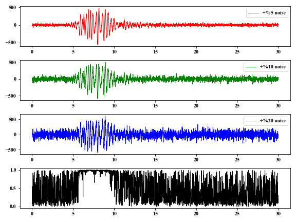
In the time window of $5-10 \ s$, the coherence $c(t)$ is approximately $1$ , because this window contains the lower-frequency coherent signals.
4. A realistic application
Some researchers utilize the PWS to accelerate the covergence of noise cross-correlation time functions (e.g., Dias et al., 2015; Dantas et al., 2018), and we use the PWS strategy to suppress the noise contaminating the noise cross-correlation functions from hurricane events. The PWS is given by the following Python code.
|
|
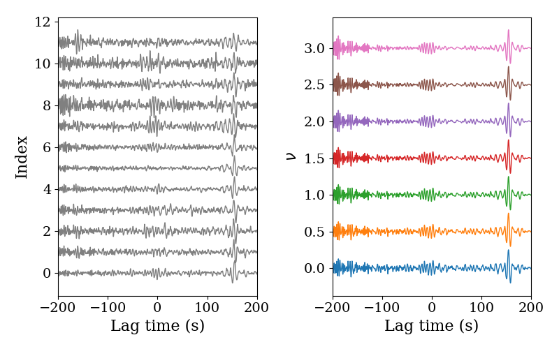
Here, we compare the stacked signals from PWS with different power numbers $\nu$ and linear stacking.
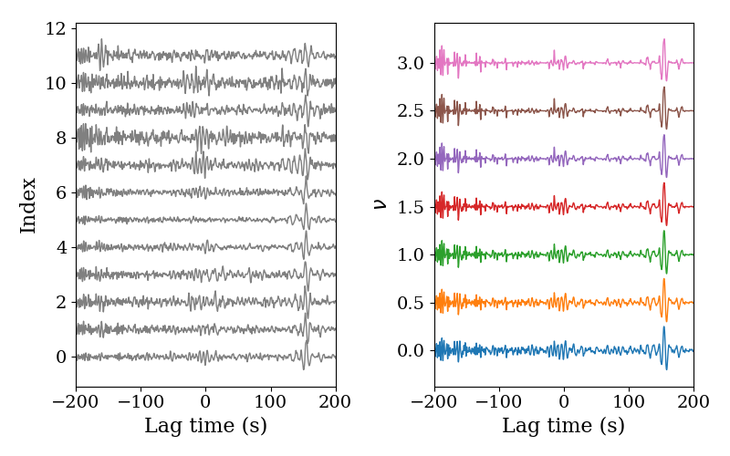
The power number $\nu$ of coherence $c(t)$ are indicated by the numbers on the right panel. Note that the SNRs become higher with the increase of the power number $\nu$. However, one must understand that the waveforms from PWS may change, especially for the larger power number $\nu$.
5 An Extension of PWS: tf-PWS
The stacked waveform using PWS changes much due to the non-linear influence. Here, Schimmel et al. (2011) have developed an extension of the PWS: tf-PWS in time-frequency domain. The steps are
(1) Transform the trace into time-frequency domain with Stockwell transform or S transform; $$ S(\tau, f)=\int_{-\infty}^{\infty}u(t)w(\tau-t, f)e^{-i2\pi ft} \tag{4}, $$ where $w(\tau-t, f)=\frac{|f|}{k\sqrt{2\pi}}e^{-f^2(\tau-t)^2/(2k^2)}$ with $k>0$ is an Gaussian window function. The new coherence function is defined by $$ c(\tau, f)=|\frac{1}{N}\sum_{n=1}^N \frac{S_n(\tau, f)e^{i2\pi ft}}{|S_n(\tau, f)|}|^\nu \tag{5}. $$ The stacked waveform with tf-PWS in time-frequency domain is $$ S_{tf-PWS}(\tau, f)=c(\tau, f)S_{linear}(\tau, f) \tag{6}, $$ where, $S_{linear}(\tau, f)$ is the linear stacking of all traces in time-frequency domain using S transform.
We apply an inverse S transform to $S_{tf-PWS}(\tau, f)$ and obtain the tf-PWS waveform $s(\tau)$.
6 An Application of tf-PWS
We use the same noise cross-correlations to check the tf-PWS. You need to install the Python library stockwell first if you want to try the following example.
|
|
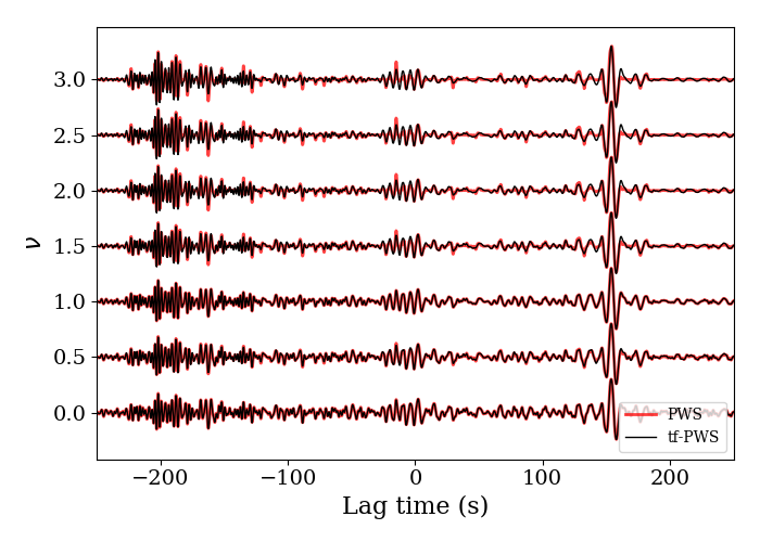
We can find that the stacked waveforms with tf-PWS do not change much but noise is suppressed. We compare the stacked waveforms with the PWS and tf-PWS, and we can see that the difference is more obvious when the power number $\nu$ increases.
References
Dias, R.C., Julià, J. & Schimmel, M. Rayleigh-Wave, Group-Velocity Tomography of the Borborema Province, NE Brazil, from Ambient Seismic Noise. Pure Appl. Geophys. 172, 1429–1449.
Dantas, Odmaksuel Anísio Bezerra, Do Nascimento, A. F. , & Schimmel, M. . (2018). Retrieval of body-wave reflections using ambient noise interferometry using a small-scale experiment. Pure & Applied Geophysics.
Schimmel, M., and H. Paulssen (1997), Noise reduction and detection of weak, coherent signals through phase weighted stacks, Geophys. J. Int., 130, 497 – 505.
M. Schimmel, E. Stutzmann2and J. Gallart. Using instantaneous phase coherence for signal extraction from ambient noise data at a local to a global scale. Geophysical Journal International(1), 494-506.
Shapiro, N. M., and M. Campillo (2004). Emergence of broadband Rayleigh waves from correlations of the ambient seismic noise, Geophys. Res. Lett. 31, no. 7, doi: 10.1029/2004GL019491.
Author Geophydog
LastMod 2021-01-16