1 Introduction

Benefiting by the installation of seismic stations, we can, to some extend, understand that how our planet Earth sings. These sounds released by our planet generate the vibration signals that can be recorded by the seismic receivers. Seismic ambient noise, which is generated by ocean infragravity waves, commonly referred to as “Hum” ($30 - 500 \ s $), microseisms ( the primary and secondary, $1 - 30 \ s$) and human noise (cultural noise, $0.1 - 1 \ s$) (Nakata et al., 2019). How to estimate the level of seismic ambient noise? The power spectral density (PSD) is usually used to describe the seismic noise spectra. Here, we briefly introduce the steps of estimating the seismic noise, some Python codes included. By the way, the PSD model of the seismic ambient noise has been introduced by Peterson (1993).

2 Basic principles

Supposing that we have a stochastic time series (randomly generated noise) $u(t)$, and the discrete form is represented as $u(n)$. The assumption that $u(t)$ is periodic is given here, we can directly estimate the its PSD as $$ p(\omega) = \frac{1}{T}|U(\omega)|^2 \tag{1}, $$ where $U(\omega)$ is the Fourier spectrum of $u(t)$, namely $U(\omega)=\int_{-T/2}^{T/2}u(t)e^{-i\omega t}dt$.

The discrete form of $p(\omega)$ is given by $$ p(k)=\frac{1}{N}|U(k)|^2 \tag{2}, $$ where, $N$ is the total data point number of $u(n)$.

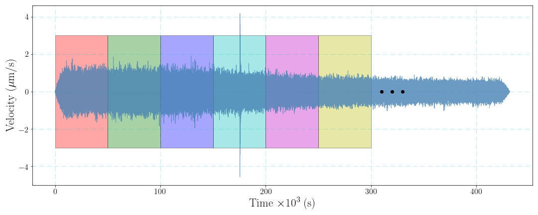
However, the seismic noise is not stochastic stable and the direct estimation method is thus not proper. One may think that we can divide the noise time series into several segments to repeat the estimations of the PSD and calculate the average PSD to obtain the final result. Indeed, this data processing will improve the stability of the PSD of the seismic noise. Here we cut the data into $M$ segments and the length of every segment is $L$, the average PSD is obtained by $$ \bar{p}(k)=\frac{1}{M}\sum_{m=1}^M[\frac{1}{L}|U_m(k)|^2] \tag{3}. $$ Similar to the idea of short time Fourier transform, window function can be also taken into consideration. Dividing data into several segments is the situation of rectangle window function. Sometimes we may use non-rectangle window function to conduct the data processing.

No overlap

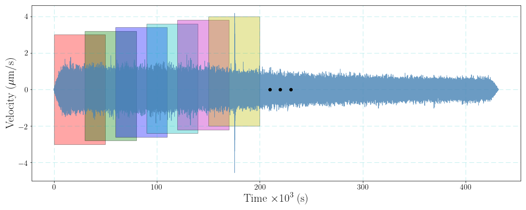
Finally, considering the data overlap can improve stability of the PSD result. The choice of the length of overlap, however, may need to tested for the perfect situation.

Overlap

3 A Realistic Example

Here we retrieve $LHZ$ component seismic noise data recoded by station $MSEY$ of network $II$ from $2018-07-29T00:00:00$ to $2018-08-02T00:00:00$ in Seychelles, a island in the Indian Ocean.

The sampling rate is $1 \ Hz$, so the maximum frequency is $0.5 \ Hz$ according to the $ Nyquist $ sampling theorem.

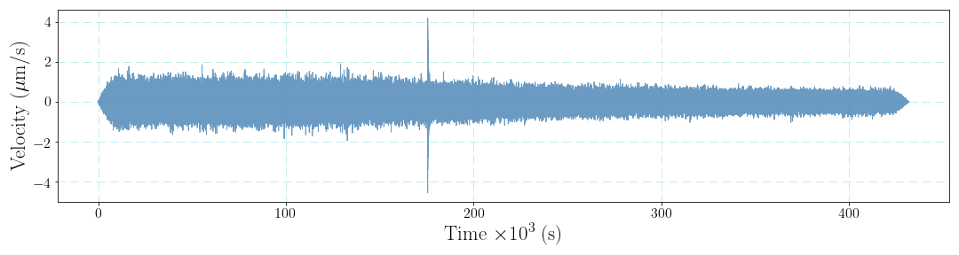
We will compare the PSD results from different estimation strategies in the following parts. Some pre-processing steps should be finished, e.g., removing mean, trend, doing tapering and removing the instrument response. The velocity waveform after removing instrument response is show as the below figure.

 1
 2
 3
 4
 5
 6
 7
 8
 9
10
11
12
13
14
15
16
17
18
19
20
21
22
23
import numpy as np
import matplotlib.pyplot as plt
from scipy.signal import savgol_filter as sgolay
from obspy import read
from scipy.signal import welch
import matplotlib

matplotlib.rcParams['text.usetex'] = True

tr = read('II.MSEY.00.LHZ.SAC')[0]
trc = tr.copy()
d = trc.data * 1e6
dt = trc.stats.delta
t = np.arange(len(d)) * dt / 1e3

plt.figure(figsize=(15, 4))
plt.plot(t, d, lw=1, color='#4682B4', alpha=0.8)
plt.xticks(fontsize=16); plt.yticks(fontsize=16)
plt.xlabel(r'Time $\times 10^3$ (s)', fontsize=23)
plt.ylabel(r'Velocity ($\mu $m/s)', fontsize=23)
plt.grid(lw=1, ls=(2, (10, 5)), color='c', alpha=0.25)
plt.tight_layout()
plt.show()

waveform

We implement a Python method to estimate the average PSD of discrete time series with dividing the data into several segments:

 1
 2
 3
 4
 5
 6
 7
 8
 9
10
11
12
13
14
15
16
17
18
19
20
21
22
23
24
25
26
def overlap_psd(tr, seg, overlap):
    if seg < overlap:
        print('Ensure segment > overlap!')
        return
    dt = tr.stats.delta; fs = 1 / dt
    over_t = (seg-overlap) * dt
    seg_t = seg * dt
    ti = 0
    p1 = np.zeros(seg)
    index = 0
    t0 = tr.stats.starttime
    t1 = t0
    while t1 < tr.stats.endtime-seg_t:
        t2 = t1 + seg_t
        trc = tr.copy()
        trc.trim(t1, t2)
        trc.data -= np.mean(trc.data); trc.detrend(); trc.taper(0.01)
        dd = trc.data
        p = np.fft.fft(dd, seg)
        p = abs(p) ** 2 / seg
        p1 += p
        t1 += over_t
        index += 1
    f1 = np.arange(seg) * fs / (seg-1)
    p1 /= index; p1 = 10 * np.log10(p1)
    return f1, p1

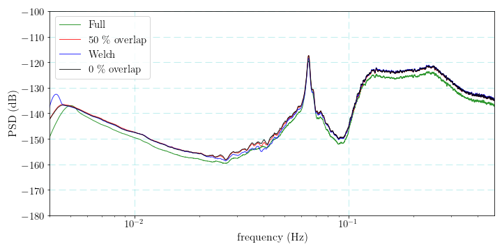
The PSD results from several estimation strategies are computed.

 1
 2
 3
 4
 5
 6
 7
 8
 9
10
11
12
13
14
15
16
17
18
19
20
21
22
23
24
25
26
27
28
29
30
31
32
33
34
35
36
37
38
39
40
41
42
43
44
45
46
# The whole window.
d0 = trc.data
n0 = len(d0)
f0 = np.arange(n0) * fs / (n0-1)
p0 = 10 * np.log10( abs(np.fft.fft(d0))**2/n0 )

# Overlapped windows.
fs = 1 / trc.stats.delta
d = trc.data
seg = 2 ** 16
overlap = seg // 2
f1, p1 = overlap_psd(trc, seg, overlap)

# Welch.
f2, p2= welch(trc.data, fs, nperseg=seg, noverlap=overlap)
p2 = 10 * np.log10(p2)

# No overlaped windows.
fs = 1 / trc.stats.delta
d = trc.data
seg = 2 ** 16
overlap = 0
f3, p3 = overlap_psd(trc, seg, overlap)

# Smoothing the PSD results with the Savitzky-Golay filter.
sl = 201
p0 = sgolay(p0, 10*sl+1, 2)
p1 = sgolay(p1, sl, 2)
p2 = sgolay(p2, sl, 2)
p3 = sgolay(p3, sl, 2)

# Plot the PSD results.
plt.figure(figsize=(15, 8))
plt.semilogx(f0, p0, lw=1, color='g', alpha=0.8, label=r'Full')
plt.semilogx(f1, p1, lw=1, color='r', alpha=0.8, label=r'50 \% overlap')
plt.semilogx(f2, p2, lw=1, color='b', alpha=0.8, label=r'Welch')
plt.semilogx(f3, p3, lw=1, color='k', alpha=0.8, label=r'0 \% overlap')
plt.legend(fontsize=20)
plt.xlim(4e-3, fs*0.48)
plt.ylim(-180, -100)
plt.xticks(fontsize=20); plt.yticks(fontsize=20)
plt.xlabel('frequency (Hz)', fontsize=25)
plt.ylabel('PSD (dB)', fontsize=25)
plt.grid(lw=1, ls=(2, (10, 5)), color='c', alpha=0.25)
plt.tight_layout()
plt.show()

PSD

4 The PSD Probability Density Function Estimation

The PSD probability density function (PSDPDF) is used to visualize the PSD of seismic noise and one can consider long-duration seismic noise data. By dividing the noise time series into many segments (overlap involved if necessary), we map every PSD curve into the PSDPDF figure. In detail, we accumulate the number of all PSD curve at every frequency value, and the probability at some power value and frequency could be obtained by dividing the cumulative number is with the sum of all numbers at this frequency.

Here we collect one-year seismic noise data recorded by a seismic station ($CASY$ in network $IU$) in Antarctica in 2020. We divide the noise time series into daily segments to compute the PSDPDF of noise at this seismic station.

 1
 2
 3
 4
 5
 6
 7
 8
 9
10
11
12
13
14
15
16
17
18
19
20
21
22
23
24
25
26
27
28
29
30
31
32
33
34
35
36
37
38
39
40
41
42
43
44
45
46
47
48
49
50
51
52
53
54
55
56
57
58
59
60
61
62
63
64
65
66
67
68
69
70
71
72
import numpy as np
import matplotlib.pyplot as plt
from scipy.signal import savgol_filter as sgolay
from obspy import read
from glob import glob
from scipy.signal import convolve2d

files = sorted(glob(r'IU.CASY*.SAC'))

nfft = 2 ** 17
nr = 251
hn = nfft // 2
psd = np.zeros((nr, hn))
p = np.zeros(hn)
for i, sac in enumerate(files):
    tr = read(sac)[0]
    fd = 10 * np.log10(abs(np.fft.fft(tr.data, nfft)) ** 2 / nfft)
    p += fd[:hn]
    for j in range(hn):
        index = int(fd[j]+250)
        if index < 0:
            index = 0
        if index > 250:
            index = 250
        psd[index, j] += 1
        
        
f1 = 5e-4; f2 = 0.45
fs = 1 / tr.stats.delta
f = np.arange(nfft) * fs / (nfft-1)
fn1 = int(f1*nfft/fs); fn2 = int(f2*nfft/fs)

nrf = 10
f = f[fn1: fn2+1]; f = f[::nrf]
P = psd[:, fn1: fn2]
pp = sgolay(p, 11, 2)
pp = pp[fn1: fn2+1] / len(files); pp = pp[::nrf]
P = P[::1, ::nrf]
sl = 2
P = convolve2d(P, np.ones((sl, sl))/sl**2, 'same')
db = np.arange(nr) - 250
P = P[50: 171]; db = db[50: 171]
for i in range(len(P[0])):
    P[:, i] /= np.sum(P[:, i])

plt.figure(figsize=(15, 8))
plt.pcolormesh(f, db, P*100, cmap='CMRmap_r')
cbar = plt.colorbar(shrink=0.75, aspect=30, pad=0.05, extend='both')
cbar.set_label(r'Probability (%)', fontsize=20)
cbar.ax.tick_params(labelsize=16)
plt.semilogx(f, pp, lw=2, color='#888888')
plt.text(2.5e-3, -125, 'Hum', size=25,
        bbox=dict(boxstyle='round',
                   ec='#333333',
                   fc='#87CEFA',
                   ))
plt.text(6e-2, -130, 'SF', size=20,
        bbox=dict(boxstyle='round',
                   ec='#333333',
                   fc='#87CEFA',
                   ))
plt.text(0.11, -115, 'DF', size=20,
        bbox=dict(boxstyle='round',
                   ec='#333333',
                   fc='#87CEFA',
                   ))
plt.xlabel('Freuqency (Hz)', fontsize=25)
plt.ylabel('Velocity PSD (dB)', fontsize=25)
plt.xticks(fontsize=20)
plt.yticks(fontsize=20)
plt.tight_layout()
plt.show()

IU.CASY PSDPDF

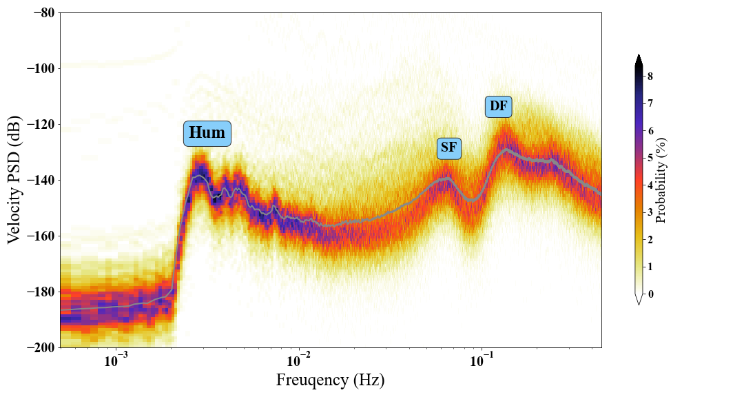
The hum, SF (single-frequency, the primary) and DF (double-frequency, the secondary) microseisms are marked on the figure. The gray curve denotes the average PSD from $366$-day ambient seismic noise data segments.

Bibliography

Nakata, Nori; Gualtieri, Lucia; Fichtner, Andreas (2019). *Seismic Ambient Noise || Noise-Based Monitoring. , 10.1017/9781108264808(9).

Peterson, J. 1993. Observations and modeling of seismic background noise. U.S. Geol. Surv. Tech. Rept., 93-322, 1–95