Geometry on a Sphere

Plane geometry is familiar to us after we got through the life at junior middle school and senior high school. Spherical geometry, however, is a little difficult for us. Here, some topics, e.g., the great-circle distance, azimuth or back-azimuth will be introduced and implemented with the Python codes in the following sections.

1 The great-circle distance

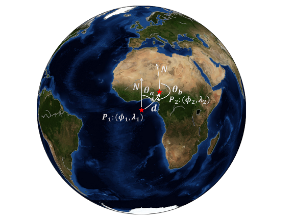
Often, we calculate the great-circle distance of given two points in geophysics, for example, the distance from the seismic station to the epicenter. Supposing that we have two geographical points, and let’s say $P_1:\ (\phi_1, \lambda_1)$ and $P_2: \ (\phi_2, \lambda_2)$, where, $\phi$ and $\lambda$ represent the latitude and longitude, respectively. Using Haversine formula, we can calculate the great-circle distance.

Geometry $$ \left \{ \begin{aligned} a &= sin^2(\frac{\Delta \phi}{2}) + cos\phi_1 \cdot cos\phi_2 \cdot sin^2(\frac{\Delta \lambda}{2}) \\
c &= 2 \cdot tan^{-1}(\frac{\sqrt{a}}{\sqrt{1-a}}) \text{ or } 2 \cdot sin^{-1}(\sqrt{a})\\
d &= c \cdot R \end{aligned} \right. \tag{1}, $$ where, $R$ is the average radius of our planet Earth, $\Delta \phi=\phi_2-\phi_1$ and $\Delta \lambda=\lambda_2-\lambda_1$. Here, we using the Python codes to give an example.

 1
 2
 3
 4
 5
 6
 7
 8
 9
10
11
12
13
14
15


import numpy as np

# The average radius of the Earth in km.
R = 6371
# The start point.
la1 = 0; lo1 = 0
# The end point.
la2 = 10; lo2 = 10
# Convertion factor from degree to radian.
d2r = np.pi / 180
dla = (la2-la1) * d2r
dlo = (lo2-lo1) * d2r
a = np.sin(dla/2) ** 2 + np.cos(la1*d2r) * np.cos(la2*d2r) * np.sin(dlo/2) ** 2
c = 2 * np.arctan2(a**0.5, (1-a)**0.5)
d1 = R * c

The implementation of finding the great-circle distance is in the Obspy library. We compare the results from above codes and the Obspy.

1
2
3
4
5


from obspy.taup.taup_geo import calc_dist_azi as cda

d2, az2, baz2 = cda(la1, lo1, la2, lo2, R, 0)
d2 *= d2r*R
print(d1, d2)

this: 1568.5205568
obspy: 1568.520556798576

$\color{red}{\text{One should note that we need to convert the degrees to radians} }$

$\color{red}{\text{ when we use trigonometric functions.}}$

2 The azimuth and back-azimuth

The azimuth or bearing is defined by the angle from the north to the great-circle arc of two geographical points. Here, we directly give the formula of calculating the azimuth $\theta$. $$ \left \{ \begin{aligned} y &= sin(\Delta \lambda) \cdot cos\phi_2 \\
x &= cos\phi_1 \cdot sin\phi_2 - sin\phi_1 \cdot cos\phi_2 \cdot cos(\Delta \lambda) \\
\alpha &= tan^{-1}\frac{y}{x} \\
\theta_a &= (\alpha \cdot 180 / \pi + 360) % 360 \end{aligned} \right. \tag{2}. $$ Exchange the order of $P_1$ and $P_2$ if one wants to calculate the back-azimuth $\theta_b$.

1
2
3
4
5
6


y = np.sin(dlo) * np.cos(la2*d2r)
x = np.cos(la1*d2r) * np.sin(la2*d2r) - np.sin(la1*d2r) * np.cos(la2*d2r) * np.cos(dlo)
th = np.arctan2(y, x)
az1 = (th / d2r + 360) % 360

print('this: ', az1, '\nobspy:', az2)

this: 44.5614514133
obspy: 44.56145141325769

3 The mid-point of two points

Now we suppose to find the mid-point $P_m: \ (\phi_m, \lambda_m)$ of the given two points, and this mid-point is defined as the half-way point along the great-circle arc between the given two points. The formula is given by $$ \left \{ \begin{aligned} b_x &= cos(\phi_2) \cdot cos(\Delta \lambda) \\
b_y &= cos(\phi_2) \cdot sin(\Delta \lambda) \\
\phi_m &= tan^{-1}(\frac{sin\phi_1+sin\phi_2}{\sqrt{(cos\phi_1+b_x)^2+b_y^2}})\\
\lambda_m &= \lambda_1 + tan^{-1}(\frac{b_y}{cos\phi_1+b_x}) \end{aligned} \right. \tag{3}. $$

1
2
3
4
5
6


bx = np.cos(la2*d2r) * np.cos(dla)
by = np.cos(la2*d2r) * np.sin(dla)

lam = np.arctan2(np.sin(la1*d2r)+np.sin(la2*d2r), ( (np.cos(la1*d2r)+bx)**2+by**2 )**0.5 ) / d2r
lom = lo1 + np.arctan2(by, np.cos(lo1*d2r)+bx) / d2r
print(lam, lom)

5.01900069786 4.9616312267

Let’s check whether this result is reasonable or not. We set a function of calculating the great-circle distance first and use it to calculate the distances of the $P_m$ between $P_1$ and $P_2$, respectively. We also write a function of calculating the azimuth from the start point to the end point.

 1
 2
 3
 4
 5
 6
 7
 8
 9
10
11
12
13
14
15
16
17
18
19
20
21


def dist(la1, lo1, la2, lo2, R=6371, km=True):
    d2r = np.pi / 180
    dla = (la2-la1) * d2r
    dlo = (lo2-lo1) * d2r
    a = np.sin(dla/2) ** 2 + np.cos(la1*d2r) * np.cos(la2*d2r) * np.sin(dlo/2) ** 2
    c = 2 * np.arctan2(a**0.5, (1-a)**0.5)
    if km:
        return R * c
    return c

def azimuth(la1, lo1, la2, lo2):
    d2r = np.pi / 180
    dla = (la2 - la1) * d2r
    dlo = (lo2 - lo1) * d2r
    y = np.sin(dlo) * np.cos(la2*d2r)
    x = np.cos(la1*d2r) * np.sin(la2*d2r) - np.sin(la1*d2r) * np.cos(la2*d2r) * np.cos(dlo)
    th = np.arctan2(y, x)
    return (th / d2r + 360) % 360

print('distance in km:', dist(la1, lo1, lam, lom), dist(lam, lom, la2, lo2))
print('azimuth:', azimuth(la1, lo1, lam, lom), azimuth(lam, lom, la2, lo2))

distance in km: 784.260278399 784.260278399

azimuth: 44.5614514133 44.7790409161

4 Intermediate point: the point on the great-circle arc with given fraction

An intermediate point $P_i: \ (\phi_i, \lambda_i)$ at arbitrary fraction $\alpha$ along the great circle path between the given two points can also be calculated. The formula is $$ \left \{ \begin{aligned} a &= \frac{ sin[(1-\alpha)\cdot\Delta] }{sin\Delta} \\
b &= \frac{ sin(\alpha \cdot \Delta) } {sin\Delta} \\
x &= a \cdot cos\phi_1 \cdot cos\lambda_1 + b \cdot cos \phi_2 \cdot cos\lambda_2 \\
y &= a \cdot cos\phi_1 \cdot sin\lambda_1 + b \cdot cos\phi_2 \cdot sin\lambda_2 \\
z &= a \cdot sin\phi_1 + b \cdot sin\phi_2\\
\phi_i &= tan^{-1}(\frac{z}{\sqrt{(x^2+y^2)}})\\
\lambda_i &= tan^{-1}(\frac{y}{x}) \end{aligned} \right. \tag{4}, $$ where, $\Delta$ is the great-circle angular distance of the given two points $P_1$ and $P_2$.

Again, we write a function of calculating the intermediate point as below. The intermediate point is $P_1$ when $\alpha=0$ and $P_2$ when $\alpha=1$.

 1
 2
 3
 4
 5
 6
 7
 8
 9
10
11
12


def im_point(la1, lo1, la2, lo2, alpha=0.5, R=6371):
    delta = dist(la1, lo1, la2, lo2, R=R, km=False)
    d2r = np.pi / 180
    la1, lo1, la2, lo2 = la1*d2r, lo1*d2r, la2*d2r, lo2*d2r
    a = np.sin((1-alpha)*delta) / np.sin(delta)
    b = np.sin(alpha*delta) / np.sin(delta)
    x = a * np.cos(la1) * np.cos(lo1) + b * np.cos(la2) * np.cos(lo2)
    y = a * np.cos(la1) * np.sin(lo1) + b * np.cos(la2) * np.sin(lo2)
    z = a * np.sin(la1) + b * np.sin(la2)
    lai = np.arctan2(z, (x**2+y**2)**0.5)
    loi = np.arctan2(y, x)
    return lai/d2r, loi/d2r

We set the fraction $\alpha=0.5$ that is the mid-point to verify our Python codes.

1

print(im_point(la1, lo1, la2, lo2, alpha=0.5, R=6371))

(5.0190006978611459, 4.9616312267025062)

5 Searching the destination point with given distance and azimuth

The destination which we term here, is the point when the great-circle distance and azimuth from the start point are given. This can be solved by $$ \left \{ \begin{aligned} \phi_d &= sin^{-1}(sin\phi_1\cdot cos\Delta+cos\phi_1 \cdot sin(\Delta) \cdot cos \theta_a) \\
\lambda_d &= \lambda_1 + tan^{-1}(\frac{sin\theta_a\cdot sin\Delta \cdot cos\phi_1} {cos\Delta-sin\phi_1\cdot sin\phi_d}) \end{aligned} \right. \tag{5}. $$

Here, we check our codes with the start point $P_1$, azimuth and the distance from $P_1$ to $P_2$.

 1
 2
 3
 4
 5
 6
 7
 8
 9
10
11


def dest_point(la1, lo1, az, delta):
    d2r = np.pi / 180
    la1 *= d2r
    lo1 *= d2r
    az *= d2r
    delta *= d2r
    lad = np.arcsin(np.sin(la1)*np.cos(delta)+np.cos(la1)*np.sin(delta)*np.cos(az))
    lod = lo1 + np.arctan2(np.sin(az)*np.sin(delta)*np.cos(la1), np.cos(delta)-np.sin(la1)*np.sin(lad))
    return lad/d2r, lod/d2r

print(dest_point(la1, lo1, 44.56145141325769, dist(la1, lo1, la2, lo2, km=False)/d2r))

(10.0, 10.0)

6 Intersection point of two great-circle paths when the start points and azimuths are given

Geometry2

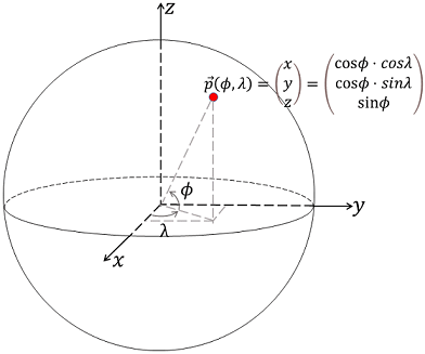
Where is the intersection point $P_i: \ (\phi_i, \lambda_i)$ of two great-circle arcs when we have two start points and corresponding azimuth? First we convert the geographical point on a sphere to Cartecian coordinate according to $$ P(\phi, \lambda) \rightarrow \left [ \begin{array}{l} & cos\phi \cdot cos\lambda \\
& cos\phi \cdot sin\lambda \\
& sin\phi \end{array} \right ] \tag{6}, $$ where, $\phi$ and $\lambda$ are latitude and longitude, respectively. With given the start point $\vec{a_0}$, azimuth $\theta_a$ and the great-circle angular distance $\Delta_a$, we can constrain the end point $\vec{a_1}$ on the great-circle arc. Similarly, we have the second great-circle arc according to these parameters: $\vec{b_0}$, $\theta_b$ and $\Delta_b$.

Let’s define two vectors, $$ \left \{ \begin{aligned} \vec{p} &= \vec{a_0} \times \vec{a_1} \\
\vec{q} &= \vec{b_0} \times \vec{b_1} \end{aligned} \right. \tag{7}. $$ A new unit vector $\vec{t}$ defined as $$ \vec{t} = \frac{\vec{p} \times \vec{q}}{|\vec{p} \times \vec{q}|} \tag{8}. $$ Four scalars are given by $$ \left \{ \begin{aligned} s_1 &= \vec{a_0} \times \vec{p} \cdot \vec{t} \\
s_2 &= \vec{a_1} \times \vec{p} \cdot \vec{t} \\
s_3 &= \vec{b_0} \times \vec{q} \cdot \vec{t} \\
s_4 &= \vec{b_1} \times \vec{q} \cdot \vec{t} \end{aligned} \right. \tag{9}, $$ and we can find the intersection point by checking whether $-s_1, s_2, -s_3$ and $s_4$ are all the same sign. The last vector $\vec{t}$ is modified by $$ \left \{ \begin{aligned} \vec{t} &= \vec{t} \ \text{ if all the signs of the above four scalars are positive} \\
\vec{t} &= -\vec{t} \ \text{ if all the signs of the above four scalars are negative} \end{aligned} \right. \tag{10}. $$

Let $x, y$ and $z$ be the components of the vector $t$, and the geographical information $(\phi, \lambda)$ of the intersection is given by $$ \left \{ \begin{aligned} \phi &= tan^{-1}(\frac{z}{\sqrt{x^2+y^2}}) \\
\lambda &= tan^{-1}(\frac{y}{x}) \end{aligned} \right. \tag{11} $$ The Python codes are

 1
 2
 3
 4
 5
 6
 7
 8
 9
10
11
12
13
14
15
16
17
18
19
20
21
22
23
24
25
26
27
28
29


def intersection(la1, lo1, la2, lo2, az1, az2, dt=180):
    d2r = np.pi / 180
    def s2c(la, lo):
        return np.array([np.cos(la*d2r)*np.cos(lo*d2r),
                         np.cos(la*d2r)*np.sin(lo*d2r),
                         np.sin(la*d2r)])
    a0 = s2c(la1, lo1); b0 = s2c(la2, lo2)
    a1 = dest_point(la1, lo1, az1, dt)
    a1 = s2c(a1[0], a1[1])
    b1 = dest_point(la2, lo2, az2, dt)
    b1 = s2c(b1[0], b1[1])

    p = np.cross(a0, a1); q = np.cross(b0, b1)
    t = np.cross(p, q); t /= np.dot(t, t)**0.5
    s1 = np.dot(np.cross(a0, p), t)
    s2 = np.dot(np.cross(a1, p), t)
    s3 = np.dot(np.cross(b0, q), t)
    s4 = np.dot(np.cross(b1, q), t)
    flag = np.array([-s1, s2, -s3, s4])
    if np.all(flag>0):
        tmp = t
    elif np.all(flag<0):
        tmp = -t
    else:
        print('No intersection!')
        return np.zeros(2)
    la = np.arctan2(tmp[2], (tmp[0]**2+tmp[1]**2)**0.5)
    lo = np.arctan2(tmp[1], tmp[0])
    return np.array([la, lo]) / d2r   

We give two start points $(0, 0), (0, -10)$, corresponding azimuths $180, 90$ degrees and great-circle angular distances $20$ degrees, and the intersection point is reasonably $(0, 0)$. Let’s check!

1

print(intersection(10, 0, 0, -10, 180, 90, dt=20))

[ 6.09219391e-16 1.21843878e-15]

The result is not strictly $(0, 0)$, and this may be caused by the computation errors.

7 The cross-track distance

The cross-track distance is defined as the distance from a point to a great-circle arc, and this was used in our research about coda interferometry. We encountered a situation that we wanted to divide the large earthquakes into several groups according to the distances of the epicenters to the great-circle paths constrained by the station pairs in coda cross-correlations.

Geometry4

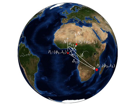
Therefore, the cross-track distance is a reasonable evaluation criteria, and it is given by $$ \Delta = |sin^{-1}[sin\Delta_{13}\cdot sin(\theta_{13}-\theta_{12})]|, \tag{12} $$

where $\Delta_{13}$ is the great-circle angular distance from $P_1$ to $P_3$, $\theta_{13}$ is the azimuth of $P_1$ to $P_3$ and $\theta_{12}$ $P_1$ to $P_2$.

Here, we set the first two geographical points $P_1:(0, -10),\ P_2:(0, 10)$ and the third point is $P_3:(10, 0)$. We know that the reasonable cross-track distance is $10$ degrees, and let’s verify that.

 1
 2
 3
 4
 5
 6
 7
 8
 9
10
11


def cross_track(la1, lo1, la2, lo2, la3, lo3, R=6371, km=True):
    d2r = np.pi / 180
    dt13 = dist(la1, lo1, la3, lo3, km=False)
    th12 = azimuth(la1, lo1, la2, lo2)
    th13 = azimuth(la1, lo1, la3, lo3)
    dt = abs(np.arcsin(np.sin(dt13)*np.sin((th13-th12)*d2r)))
    if km:
        return dt * R
    return dt / d2r

print(cross_track(0, -10, 0, 10, 10, 0, km=False))

10.0

8 The closest point to the pole(s)

First give the latitude $\phi$ of the start point and azimuth $ \theta$, and the latitude on this great-circle path can be solved by $$ \phi_m=cos^{-1}(|sin\theta \cdot cos\phi|) \tag{13}, $$ and this can derived from Clairaut’s formula.

Bibliography

http://www.movable-type.co.uk/scripts/latlong.html
https://enrico.spinielli.net/2014/10/19/understanding-great-circle-arcs_57/
Author Geophydog
LastMod 2021-03-02