Short background
Ambient noise tomography of regional and continental scales is much benefited from
the system composed of the atmosphere, ocean and the solid earth. Ambient noise below
1Hz is largely due to oceans, and interactions between ocean waves and/or the sea floor
generate pressure impulse propagating into the solid earth. Land seismic stations are seizing
seismic waves which originating from microseisms, and these seismic waves include surface waves
and body waves. Individuals can easily retrieve surface waves from ambient noise cross-correlations.
Body wave extraction from ambient noise, however, remains difficult. We often explore body waves from
ambient noise using array stacking techniques for array stacking leads to high signal-to-noise ratios.
Here we perform the body wave source location utilizing beamforming and back-projection methods,
and we process one-day seismic recordings by a seismic array in China, which reveals that the source location
is in the North Atlantic Ocean, the south of Iceland.
Data and Methods
We collect one-day continuous seismic data of vertical component(here BHZ, 2008-03-10) recorded by a seismic array nearly in
the center part of China (see the following figure), and compute the cross-spectral matrix using one-hour length
segment with a overlap of 50% (1800 seconds):
$$
C(\omega) = \frac{1}{N}\sum_{n=1}^N\boldsymbol{u}_n(\omega) \cdot \boldsymbol{u}_n^H(\omega), \tag{1}
$$
in which, $\boldsymbol{u}_n(\omega)=[u^1_n(\omega), u^2_n(\omega), \cdots, u^M_n]^T$ is the Fourier spectra
of the $n_{th}$ segment data recorded by $M$ stations, $H$ denotes Hermitian transpose, and $N$ is the total number of data segments.
Then we create steering vector as follows,
$$
\boldsymbol{a}(\omega; \boldsymbol{s}, \boldsymbol{x}) = [e^{-i\omega \boldsymbol{s} \cdot \boldsymbol{x}_1}, e^{-i\omega \boldsymbol{s} \cdot \boldsymbol{x}_2}, \cdots, e^{-i\omega \boldsymbol{s} \cdot \boldsymbol{x}_M}]^T, \tag{2}
$$
where, $\boldsymbol{s}$ and $\boldsymbol{x}_m$ separately indicate horizontal slowness (ray parameter for body waves) and position of the $m_{th}$ station.
The beam power is given by
$$
B(\omega; \boldsymbol{s}) = \boldsymbol{a}^H \boldsymbol{C}(\omega) \boldsymbol{a}. \tag{3}
$$
For more details about beamforming, someone can refer to this blog.
An Example of Locating the distant P wave source
We first import required Python libraries.
1
2
3
4
5
6
7
8
|
import numpy as np
import matplotlib.pyplot as plt
from obspy import read
from glob import glob
from mpl_toolkits.basemap import Basemap
from scipy.signal.windows import hann
import matplotlib as mpl
from obspy.taup import TauPyModel
|
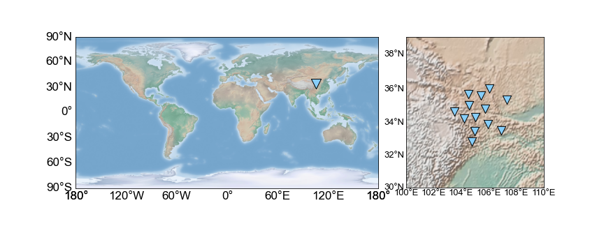
The 13 seismic stations are installed in the center part of China, and we collect the data of March 10, 2008 to perform this work.
 1
 2
 3
 4
 5
 6
 7
 8
 9
10
11
12
13
14
15
16
17
18
19
20
21
22
23
24
25
26
27
28
29
30
31
32
33
34
35
|
files = sorted(glob('2008-03-10/*BHZ.SAC'))
sta = {}
with open('X4_IRIS_BHZ.txt', 'r') as fin:
    for line in fin.readlines():
        tmp = line.strip().split('|')
        sta[tmp[1]] = [float(tmp[3]), float(tmp[2])]
xy = []
for f in files:
    tmp = f.split('/')[-1].split('.')[1]
    xy.append(sta[tmp])
xy = np.array(xy)

plt.figure(figsize=(12, 4.5))
plt.subplot2grid((1, 3), (0, 0), rowspan=1, colspan=2)
bmap1 = Basemap(projection='cyl', lon_0=0)
bmap1.shadedrelief(scale=0.2)
xx, yy = bmap1(106, 34)
bmap1.scatter(xx, yy, marker='v', s=200, facecolor='#87CEFA', edgecolor='k', lw=1, alpha=1)
bmap1.drawmeridians(meridians=np.linspace(-180, 180, 7),
                  labels=[0, 0, 0, 1], color='none', fontsize=17)
bmap1.drawparallels(circles=np.linspace(-90, 90, 7),
                  labels=[1, 0, 0, 0], color='none', fontsize=17)

plt.subplot2grid((1, 3), (0, 2), rowspan=1, colspan=1)
bmap2 = Basemap(projection='merc', llcrnrlat=30, llcrnrlon=100,
              urcrnrlon=110, urcrnrlat=39)
bmap2.shadedrelief(scale=1)
xx, yy = bmap2(xy[:, 0], xy[:, 1])
bmap2.drawcoastlines(color='gray')
bmap2.scatter(xx, yy, marker='v', s=150, facecolor='#87CEFA', edgecolor='k', lw=1, alpha=1)
bmap2.drawmeridians(meridians=np.linspace(100, 110, 6),
                  labels=[0, 0, 0, 1], color='none', fontsize=13)
bmap2.drawparallels(circles=np.linspace(30, 40, 6),
                  labels=[1, 0, 0, 0], color='none', fontsize=13)
plt.show()
|
It is worth noting that we compute the beam power in Cartesian coordinate system while we only have the longitudes and latitudes of these stations.
Thus, we have to convert these longitudes and latitudes to Cartesian coordinates, so we define the following useful functions.
 1
 2
 3
 4
 5
 6
 7
 8
 9
10
11
12
13
14
15
16
17
18
19
20
21
22
23
24
25
26
27
28
29
30
31
32
33
34
35
36
37
38
|
def distance(la1, lo1, LA2, LO2, R=6371):
    d2r = np.pi / 180
    dla = (LA2-la1) * d2r
    dlo = (LO2-lo1) * d2r
    a = np.sin(dla/2) ** 2 + np.cos(la1*d2r) * np.cos(LA2*d2r) * np.sin(dlo/2) ** 2
    c = 2 * np.arctan2(a**0.5, (1-a)**0.5)
    return R * c * 1e3

def azimuth(la1, lo1, LA2, LO2):
    d2r = np.pi / 180
    dla = (LA2 - la1) * d2r
    dlo = (LO2 - lo1) * d2r
    y = np.sin(dlo) * np.cos(LA2*d2r)
    x = np.cos(la1*d2r) * np.sin(LA2*d2r) - np.sin(la1*d2r) * np.cos(LA2*d2r) * np.cos(dlo)
    th = np.arctan2(y, x)
    return (th / d2r + 360) % 360

def lola2xy(xy):
    n = xy.shape[0]
    lo0 = xy[:, 0].mean()
    la0 = xy[:, 1].mean()
    dist = distance(la0, lo0, xy[:, 1], xy[:, 0])
    az = azimuth(la0, lo0, xy[:, 1], xy[:, 0]) * np.pi / 180
    new_xy = np.zeros_like(xy)
    new_xy[:, 0] = np.sin(az) * dist
    new_xy[:, 1] = np.cos(az) * dist
    return new_xy
def process_data(d, operator, p=0.01):
    nd = len(d)
    pn = int(nd*p)
    h = hann(2*pn)
    d -= d.mean()
    d[:pn] *= h[:pn]
    d[-pn:] *= h[-pn]
    fd = np.fft.fft(d)
    fd /= np.convolve(np.abs(fd), operator, 'same')
    fd[np.isnan(fd)] = 0.
    return fd
|
We need to estimate the average cross-spectral matrix of seismic data by this array before compute the beam power.
 1
 2
 3
 4
 5
 6
 7
 8
 9
10
11
12
13
14
15
16
17
18
19
20
21
22
23
24
25
26
27
28
29
30
31
32
33
34
35
36
37
38
39
40
|
st = read('2008-03-10/*BHZ.SAC')
utcb = st[0].stats.starttime
utce = st[0].stats.endtime
dt = st[0].stats.delta; fs = 1 / dt
xy = []
for tr in st:
    if utcb > tr.stats.starttime:
        utcb = tr.stats.starttime
    if utce < tr.stats.endtime:
        utce = tr.stats.endtime
    xy.append(sta[tr.stats.station])
xy = np.array(xy)
xy = lola2xy(xy)
n = xy.shape[0]
nd = int((utce-utcb)/dt)
data = np.zeros((n, nd+50))
for ti, tr in enumerate(st):
    n0 = int((tr.stats.starttime-utcb)/dt)
    data[ti, n0: n0+tr.stats.npts] = tr.data

pt = 3600; pn = int(pt/dt); on = pn // 2
hn = 15; operator = np.ones(hn*2+1) / (hn*2+1)
tmp_data = []
n1 = 0
while n1 < data.shape[1]-pn:
    tmp = []
    n2 = n1 + pn
    for i in range(n):
        tmp.append(process_data(data[i, n1:n2], operator))
    tmp_data.append(tmp)
    n1 += on
tmp_data = np.array(tmp_data)
f1 = 1 / 9; f2 = 1 / 5
fn1 = int(f1*pn/fs); fn2 = int(f2*pn/fs); nf = fn2 - fn1 +1
c = np.zeros((nf, n, n), dtype=complex)
u = np.zeros((n, 1), dtype=complex)
for i in range(fn1, fn2+1):
    for j in range(tmp_data.shape[0]):
        u[:, 0] = tmp_data[j, :, i]
        c[i-fn1] += u @ np.conjugate(u.T)
|
Now we compute the beam power using formula $(1)$ to estimate the back-azmith and corresponding ray parameter of the potential body wave.
 1
 2
 3
 4
 5
 6
 7
 8
 9
10
11
12
13
14
15
16
|
s1 = 0; s2 = 10; ns = 101
g = 111194.92664455
s = np.linspace(s1, s2, ns) / g
b1 = 0; b2 = 360; nb = 181
b = np.linspace(b1, b2, nb) / 180 * np.pi
p1 = np.zeros((ns, nb), dtype=complex)
a = np.zeros((n, 1), dtype=complex)
for i in range(ns):
    for j in range(nb):
        shift = -s[i] * (np.sin(b[j])*xy[:, 0] + np.cos(b[j])*xy[:, 1])
        for k in range(fn1, fn2+1):
            w = 2 * np.pi * k * fs / pn
            a[:, 0] = np.exp(-1j*w*shift)
            cc = c[k-fn1].copy(); cc /= np.abs(cc); cc[np.isnan(cc)] = 0.
            p1[i, j] += np.conjugate(a.T) @ cc @ a
p1 = np.abs(p1) / nf / n**2
|
Someone may find that we normalize the beam power using the number of frequency points and the number of stations, which results in
the coherence of signals caught by this array.
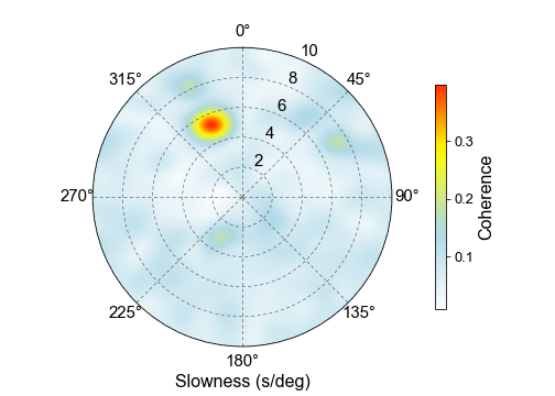
The maximum of backazimuth-slowness beam coherence panel suggests that the signal source comes from the direction ranging 315-360 degress with horizonral slowness ranging 4-6 sec/degree, and thus we identify this seismic phase as P wave. We calculate the ray parameter of P wave using the taup module, and the slowness-distance curve is shown by the following figure.
 1
 2
 3
 4
 5
 6
 7
 8
 9
10
11
12
13
14
15
16
17
18
19
20
21
22
|
model = TauPyModel(model='iasp91')
dd = 0.02
d = np.arange(0, 95+dd, dd)
pw = np.zeros((len(d), 2))
phase = ['P']
for i in range(len(d)):
    ar = model.get_travel_times(source_depth_in_km=0,
                                  distance_in_degree=d[i],
                               phase_list=phase)
    pw[i] = np.array([d[i], ar[0].ray_param])
pw[:, 1] = pw[:, 1] * np.pi / 180

plt.figure(figsize=(8, 4))
plt.plot(pw[:, 0], pw[:, 1], lw=2.5, color='#00BFFF')
plt.xlabel('Distance (degree)', fontsize=18)
plt.ylabel('Ray parameter (sec/degree)', fontsize=18)
plt.gca().tick_params(labelsize=15)
plt.xlim(30, 95)
plt.ylim(4, 10)
plt.grid(ls=(10, (6, 5)))
plt.title('Ray parameter of seismic phase P', fontsize=17)
plt.show()
|
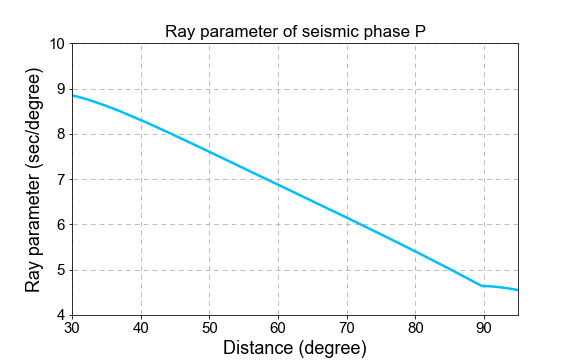
According to the beam coherence and the slowness-distance curve of P wave, we estimate that the distance between the source location the seismic array center is about 70 degrees. We utilize grid-searching rule to find the source location by projecting the backazimuth-slowness beam coherence to geographical coordinates.
 1
 2
 3
 4
 5
 6
 7
 8
 9
10
11
12
13
14
15
16
17
18
19
20
21
22
23
24
25
26
27
28
29
30
31
32
33
34
35
36
37
38
39
40
41
42
43
44
45
46
47
48
49
50
51
52
53
54
55
56
57
58
|
def distance_matrix(la1, lo1, LA2, LO2):
    d2r = np.pi / 180
    dla = (LA2-la1) * d2r
    dlo = (LO2-lo1) * d2r
    a = np.sin(dla/2) ** 2 + np.cos(la1*d2r) * np.cos(LA2*d2r) * np.sin(dlo/2) ** 2
    c = 2 * np.arctan2(a**0.5, (1-a)**0.5)
    return c * 180 / np.pi

def azimuth_matrix(la1, lo1, LA2, LO2):
    d2r = np.pi / 180
    dla = (LA2 - la1) * d2r
    dlo = (LO2 - lo1) * d2r
    y = np.sin(dlo) * np.cos(LA2*d2r)
    x = np.cos(la1*d2r) * np.sin(LA2*d2r) - np.sin(la1*d2r) * np.cos(LA2*d2r) * np.cos(dlo)
    th = np.arctan2(y, x)
    return (th / d2r + 360) % 360

xy = []
for tr in st:
    xy.append(sta[tr.stats.station])
xy = np.array(xy)
lo0 = xy[:, 0].mean()
la0 = xy[:, 1].mean()
ns, nb = p1.shape
ss = np.linspace(0, 10, ns)
bb = np.linspace(0, 360, nb)
ds = ss[1] - ss[0]
db = bb[1] - bb[0]
lo1 = -180; lo2 = 180; nlo = 181
la1 = -90; la2 = 90; nla = 91
lo = np.linspace(lo1, lo2, nlo)
la = np.linspace(la1, la2, nla)
LO, LA = np.meshgrid(lo, la)
AZ = azimuth_matrix(la0, lo0, LA, LO)
DIST = distance_matrix(la0, lo0, LA, LO)
bp = np.zeros((nla, nlo))
for i in range(nla):
    for j in range(nlo):
        index = np.argmin(np.abs(DIST[i, j]-pw[:, 0]))
        if np.abs(DIST[i, j]-pw[index, 0]) > 0.05 or pw[index, 1] > ss.max():
            continue
        si = int((pw[index, 1]-ss.min())/ds)
        ai = int((AZ[i, j]-bb.min())/db)
        bp[i, j] = p1[si, ai]

plt.figure(figsize=(12, 6))
bmap = Basemap(projection='cyl', lon_0=0)
plt.contourf(LO, LA, bp, cmap=cmap, levels=101)
cbar = plt.colorbar(shrink=0.8)
cbar.ax.tick_params(labelsize=15)
cbar.set_label('Cohenrence', fontsize=15)
bmap.fillcontinents(color='#3CB371')
bmap.drawcoastlines(linewidth=0.3, color='gray')
xx, yy = bmap(lo0, la0)
bmap.scatter(xx, yy, marker='v', s=150, facecolor='b', alpha=0.6, zorder=2)
bmap.drawparallels(circles=np.linspace(-90, 90, 7), labels=[1, 0, 0, 0], fontsize=17, color='none')
bmap.drawmeridians(meridians=np.linspace(-180, 180, 9), labels=[0, 0, 0, 1], fontsize=17, color='none')
plt.show()
|
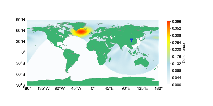 This back-projection result shows that the possible source location is in the North Atlantic Ocean, which may relate to the irregular topography of the middle ocean rige in this place.
Perspective
We use this simple example to explain the process of using body waves from ambient noise cross-correlations to investigate the potential source locations of these indentified seismic phases. Indeed, it still holds many mysteries to reveal in the seismic ambient noise world. Thus, we will continue the journey of exploring the coupling process among the atmosphere, oceans and our solid planet Earth.
