The Journey to Digital Filter Design: Low-pass Filter

Contents
Butterworth filters
$$ |H(w)|^2=\frac{1}{1+( \frac{tan\frac{\omega}{2}} {tan\frac{\omega_c}{2}})^{2N}} \tag{1} $$
Low-pass filter
Given the attenuation values $A_c$ and $A_r$ at cut-off frequencies $\omega_c$
and $\omega_r$, respectively, we first calculate the orders $N$ of filter.
We know,
$$
\begin{aligned}
A_r &= -20lg|H(\omega_s)|\\
&= -20lg\frac{1}{\sqrt{1+(\frac{tan\frac{\omega _r}{2}}{\frac{\omega_c}{2}})^{2N}}}
\end{aligned} \tag{2},
$$
and the orders $N$ is given by
$$
N = \frac{1}{2}\frac{lg(10^{\frac{A_r}{10}}-1)}{lg(\frac{tan\frac{\omega_r}{2}}{tan\frac{\omega_c}{2}})} \tag{3}.
$$
However, if you give the filter orders $N$, it can control the width of transition band of the filter.
We rewrite eq. $(1)$ as
$$
|H(\omega)|^2 = \frac{tan^{2N}\frac{\omega_c}{2}}{tan^{2N}\frac{\omega_c}{2}+tan^{2N}{\frac{\omega}{2}}} \tag{4}
$$
and according to the $Euler’s$ formula $e^{j\theta}=cos\theta+jsin\theta$, we have
$$
\begin{aligned}
tan\frac{\omega}{2} &= \frac{sin\frac{\omega}{2}}{cos\frac{\omega}{2}}\\
&= \frac{1}{j}\frac{ e^{j\frac{\omega}{2}}-e^{-j\frac{\omega}{2}} } { e^{j\frac{\omega}{2}}+e^{-j\frac{\omega}{2}} }\\
&= \frac{1}{j}\frac{ 1-e^{-j\omega} } { 1+e^{-j\omega} }
\end{aligned} \tag{5}.
$$
Let $z=e^{-j\omega}$, and combine eq. $(5)$ to yield
$$
|H(z)|^2 = \frac{tan^{2N}\frac{\omega_c}{2}} {tan^{2N}\frac{\omega_c}{2}+(-1)^N(\frac{1-z^{-1}}{1+z^{-1}})^N} \tag{6}.
$$
We know there are $N$ repeated zeros, namely, $-1$, of this transfer function and we calculate the poles as follows.
$$
q_k=
\frac{1-z_k^{-1}}{1+z_k^{-1}}=
\begin{cases}
&tan\frac{\omega_c}{2}e^{j\frac{2k+1}{2N}\pi}, \text{ for } N \text{ is even, and }k=0, 1, 2, \cdots, 2N-1;\\
&tan\frac{\omega_c}{2}e^{j\frac{k}{N}\pi}, \text{ for } N \text{ is odd and }k=0, 1, 2, \cdots, 2N-1.
\end{cases} \tag{7}.
$$
We get
$$
z_k = \frac{1+q_k}{1-q_k} \tag{8}.
$$
Lastly, the transfer function can be calculated by
$$
H(z) = \frac{1}{2^N}\frac{\prod_{|z_k|<1}(1-z_k)(1+z^{-1})^N}{\prod_{|z_k|<1}(1-z_kz^{-1})} \tag{9}.
$$
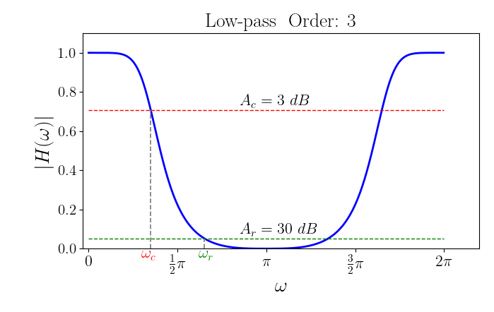
Here, we separately give attenuation values $3 \ dB$ and $30 \ dB$ at cut-off frequency $\omega_c$ and
stop frequency $\omega_r$ to show the frequency response.
We give a python code example of implementing a low-pass filter and compare this result with that filtered by the butterworth filter in scipy.
|
|
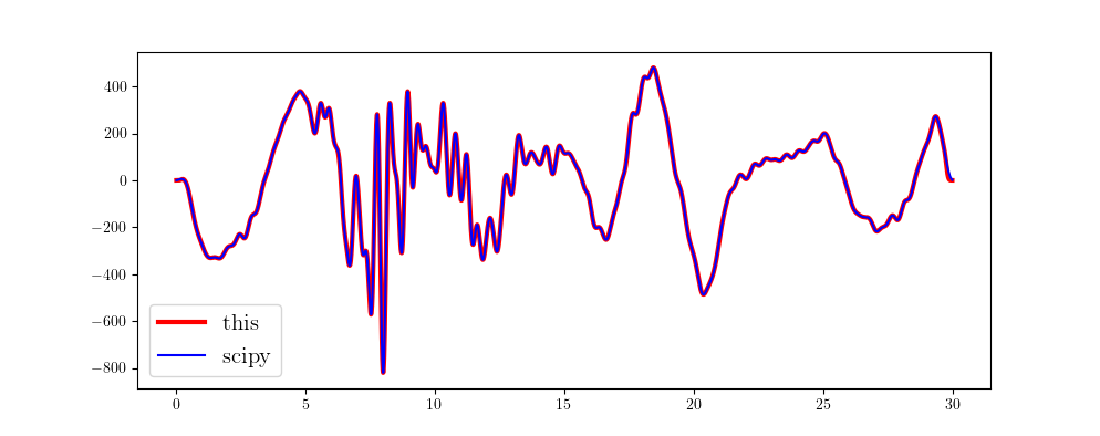 This result perfectly agrees with that in scipy, doesn’t it?
Author Geophydog
LastMod 2020-09-11