Fourier Transform

Contents
1 Introduction
The $Fourier \ Transform$ convert the signal in one domain to another domain, for instance from time domain to frequency domain. The definition of $Fourier \ Transform$ is given by $$ X(\omega) = \int_{-\infty}^\infty x(t)e^{-i \omega t} \tag{1}. $$
For the operation in programming, we need its discrete form, namely, $$ X(k) = \sum_{n=0}^{N-1}x(n) e^{\frac{-i2\pi kn}{N}} \tag{2}, $$ where, $k$ is the index of the $k_{th}$ frequency point, and we can find the $k_{th}$ frequency like this $$ f_k = \frac{kf_s}{N} \tag{3}, $$ $f_s$ is sampling rate of signal and $f_s=\frac{1}{\Delta t}$.
|
|
Actually, we have
$$
X(k) = X^*(N-k) \tag{4},
$$
where, $^*$ means the complex conjugate. Here, we show how how eq. $(4)$ comes.
$$
\begin{aligned}
X(N-k) &= \sum_{n=0}^{N-1}x(n)e^{-\frac{-i2\pi (N-k)n}{N}}\\
&= \sum_{n=0}^{N-1}x(n)e^{\frac{-i2\pi N}{N}}e^{\frac{i2\pi kn}{N}}\\
&= \sum_{n=0}^{N-1}x(n)e^{\frac{i2\pi kn}{N}}\\
&= X^*(k)
\end{aligned} \tag{5}.
$$
Eq. $(4)$ suggests that we only need to compute the first half of
$X(k), k=0, 1, 2, \cdots, \frac{N}{2}$.
2 FFT in Python
However, we just call the methods of libraries Numpy and Scipy in Python to implement $Fourier \ Transform$ as follows,
|
|
3 Code demo
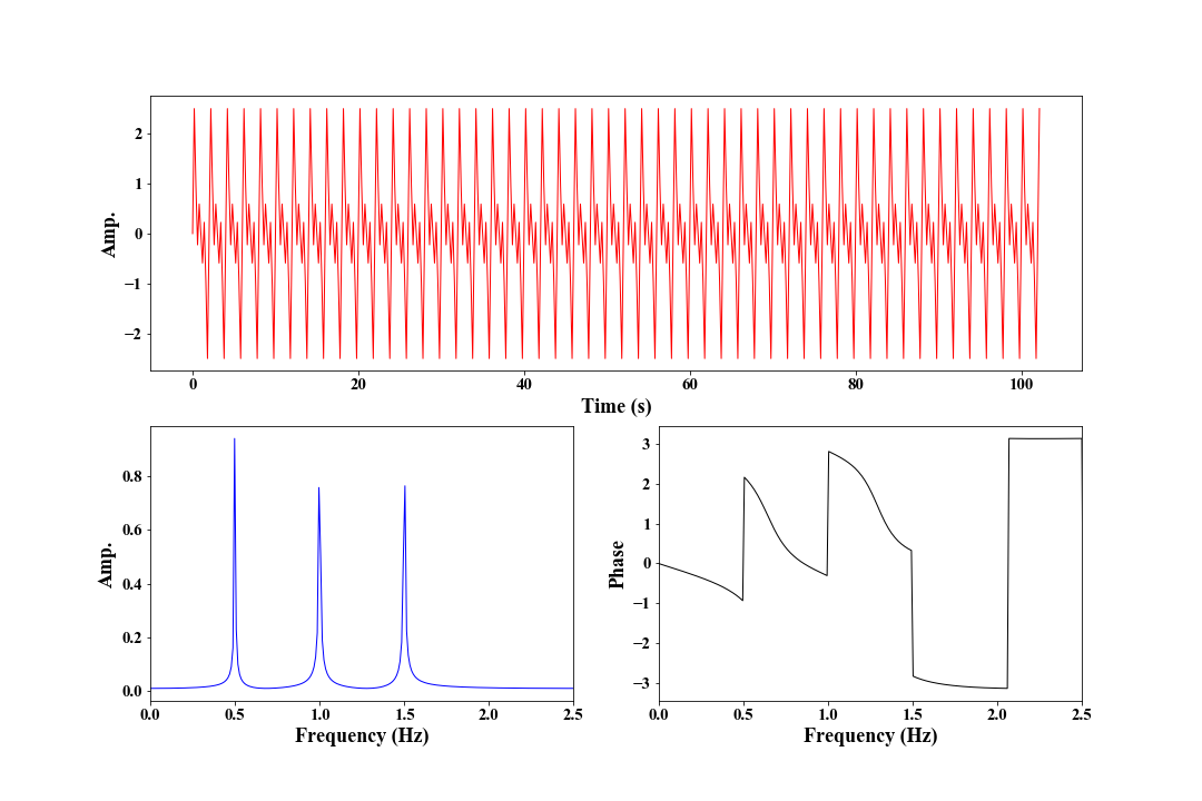
Here, we give an example to show how to convert a real signal in time domain to frequency domain.
|
|
The following figure shows the FFT of $x$.
Author Geophydog
LastMod 2020-09-03